1 Introduction

Memory is a key ingredient in our thinking and learning process. However, the understanding of learning and memories is still very limited. In 1921, Richard Semon described the idea of a memory engram, the neurophysiological trace of a memory. Nowadays, working memory is usually characterized by persistent neuron activity (Barak and Tsodyks, 2014). Recent study (Fiebig and Lansner, 2017) modeled this persistent activity with a partly plastic network and synaptic plasticity.

However, synaptic plasticity is limited to changing the weights of already existing connections and prohibits the formation of new synapses between neurons. A memory engram, e.g., in the form of a strongly interconnected group of neurons, could represent an abstract memory. If we now want to form an association with another memory in the form of a memory engram, we are limited to strengthening existing synapses with synaptic plasticity alone. We cannot build an association if there is no or only sparse connectivity between these two engrams. Moreover, ignoring structural plasticity limits the storage capacity of the brain drastically (Chklovskii et al., 2004), and structural plasticity can overcome both problems. An alternative for a model using only synaptic plasticity is to use all-to-all connectivity, but this is impractical for large networks. Additionally, recent study showed that structural plasticity also plays an essential role in the biology of memory formation (Butz et al., 2009; May, 2011; Holtmaat and Caroni, 2016) and especially long-term memory, on the other hand, is usually characterized by silent synapses (Gallinaro et al., 2022).

While most structures (Kalisman et al., 2005; Mizrahi, 2007) and synapses in the developed brain remain stable, there is evidence that learning (Holtmaat and Svoboda, 2009) and sensory input leads to an increased synapse turnover, growth of dendritic spines, and axonal remodeling (Barnes and Finnerty, 2010). For example, the alternate trimming of whisker hair of mice leads to a changed sensory input and an increased dendritic spine turnover (Trachtenberg et al., 2002), with 50% of the formed spines becoming stable. Another example is the change in the brain's gray matter when adults learn juggling (Boyke et al., 2008). Recently, it was proposed that synaptic plasticity plays a vital role in memory consolidation (Butz et al., 2009; Caroni et al., 2012; Holtmaat and Caroni, 2016). This is the process of transmitting information from the short-term memory into the long-term memory. First, learning increases the synaptic turnover and the formation of vacant synaptic elements (Butz et al., 2009; Holtmaat and Svoboda, 2009; Caroni et al., 2012). Synaptic elements are dendritic spines and axonal boutons, which, if unoccupied, generate potential synapses (Stepanyants et al., 2002). Some potential synapses later materialize, forming actual new synapses (Butz et al., 2009; Caroni et al., 2012). The correlation between spine stabilization and the performance of animals in tests (Xu et al., 2009) supports this hypothesis further. Moreover, when newly formed synapses during training are impaired, the performance of the animal decreases (Hayashi-Takagi et al., 2015), indicating that the formation of new synapses is essential for learning. However, how the learning process interacts with the increased turnover and stabilization of specific spines, without overall modification of the structures in the brain, remains unclear (Caroni et al., 2012).

Dammasch (1990) proposed the idea of forming memory engrams based on structural plasticity. Recently, Gallinaro et al. (2022) developed a model that can form silent memory engrams with only structural plasticity on a homeostatic basis. They showed that a homeostatic rule implicitly models a Hebbian learning rule and demonstrated this principle with a conditioned learning paradigm. However, their model connects neurons uniformly at random, making the simultaneous formation of clustered neurons as distinct memory engrams impossible. The stimulation of multiple memory engrams at once would lead to one single large memory engram instead of multiple small ones, which differs from the brain, where different regions are active simultaneously without interfering with one another. We extended their work with a more neurophysiological accurate approach by connecting neurons depending on their distance and forming memory engrams simultaneously. We simulated 4 million neurons with 343 engrams, enormously increasing the number of simulated neurons and memory engrams simulated with homeostatic structural plasticity. We showed that the engrams do not interfere with each other.

The structure of the model underlying our simulation draws inspiration from the human cortex, which is organized in columns further subdivided into minicolumns (Mountcastle, 1997). Each of these minicolumns consists of excitatory pyramid cells that act as a group for a specific feature depending on the cortex area. For example, a minicolumn in the visual cortex represents the orientation of an object in a visual field (Hubel and Wiesel, 1962). The different minicolumns combined comprise a hypercolumn that enables encoding all orientations for a certain spot on the retina. Similar organizations can be found in the auditory cortex (Reale and Imig, 1980) and the somatosensory cortex (Ruben et al., 2001). The columns of higher associative cortices represent more complex features such as colors (Hadjikhani et al., 1998), objects (López-Aranda et al., 2009), or persons (Downing and Peelen, 2011). In our study, we adopted the cortical organization of the associative cortices, where complex features can be learned and represented in a column. Hence, we split our network into boxes that represent a column. Each column represents a feature that acts independently from neighboring columns, and, therefore, all columns can be active simultaneously. In our example with the visual cortex, two neighboring columns encode an orientation for their field of view, respectively, without interference.

Our contributions are:

• We increased the neurophysiological plausibility of homeostatic memory models, which enables us to model cortical-like structures.

• Our model maintains the introduced structure of the cortical columns without additional constraints on how the neurons can connect.

• We formed multiple ensembles in parallel without unwanted interference between them. This is comparable to the brain with its many concurrent activities.

2 Materials and methods

In the experiment, we followed the study by Gallinaro et al. (2022), modeling a conditioned learning paradigm. In a conditioned learning paradigm, a subject learns the relationship between an unconditioned stimulus and a neutral stimulus. Before the experiment, the subject shows an unconditioned reaction to the unconditioned stimulus. During the experiment, both unconditioned (e.g., food) and neutral stimuli (e.g., bell) are presented simultaneously. After the experiment, the subject shows the same previously unconditioned (now conditioned) reaction (e.g., salivating) for the previously neutral (now conditioned) stimulus. At the level of neuronal networks, we modeled a stimulus by stimulating neurons and a reaction as the firing of a downstream, so-called readout, neuron. We split the whole population into boxes of equal side lengths and divided the neurons within each box into four distinct neuron ensembles: Unconditioned stimulus (US), conditioned stimulus 1 (C1), conditioned stimulus 2 (C2), and the rest. We added a single readout neuron (R) to each box that is fully connected to the neurons in the ensemble US with static connections (Figure 1) to monitor the unconditioned reaction of the network. With these neuron ensembles, we can model a conditioned learning paradigm by representing a neuron ensemble with a stimulus. Similar to the conditioned learning paradigm, where an unconditioned learning stimulus is presented at the same time as a conditioned stimulus and, therefore, learns a relationship between them, the network shall learn a relationship between US and C1 within each box. However, there should be no relationship associated with C2 or across different boxes, as C2 acts as our control ensemble. To accomplish this, we stimulated the ensembles US and C1 together. We performed these stimulations simultaneously for every memory that we wanted to learn.

Figure 1. Initial setup of our model network as a 2D simplification with 2 × 2 boxes. We split the boxes into equally sized boxes and grouped a subset of neurons from each box in three equally sized ensembles representing the unconditional stimulus (US), the first conditional stimulus (C1), and the second conditional stimulus (C2). The neurons of the ensemble US are fully connected with an additional readout neuron (R). The remaining neurons did not belong to any ensemble.

2.1 Model of structural plasticity

The Model of Structural Plasticity (MSP) (Butz and van Ooyen, 2013) enables structural plasticity based on a homeostatic mechanism. Each neuron controls its excitability and, therefore, the number of synapses based on its calcium concentration, which acts as a proxy for its firing rate. An approximation of MSP (Rinke et al., 2018; Czappa et al., 2023) reduced the model's computational complexity from O(n2) to O(nlogn), which enabled simulations with up to 109 neurons. Using current technology, human-scale simulations with 1011 neurons are possible in principle. We provide all model parameters in Table 1.

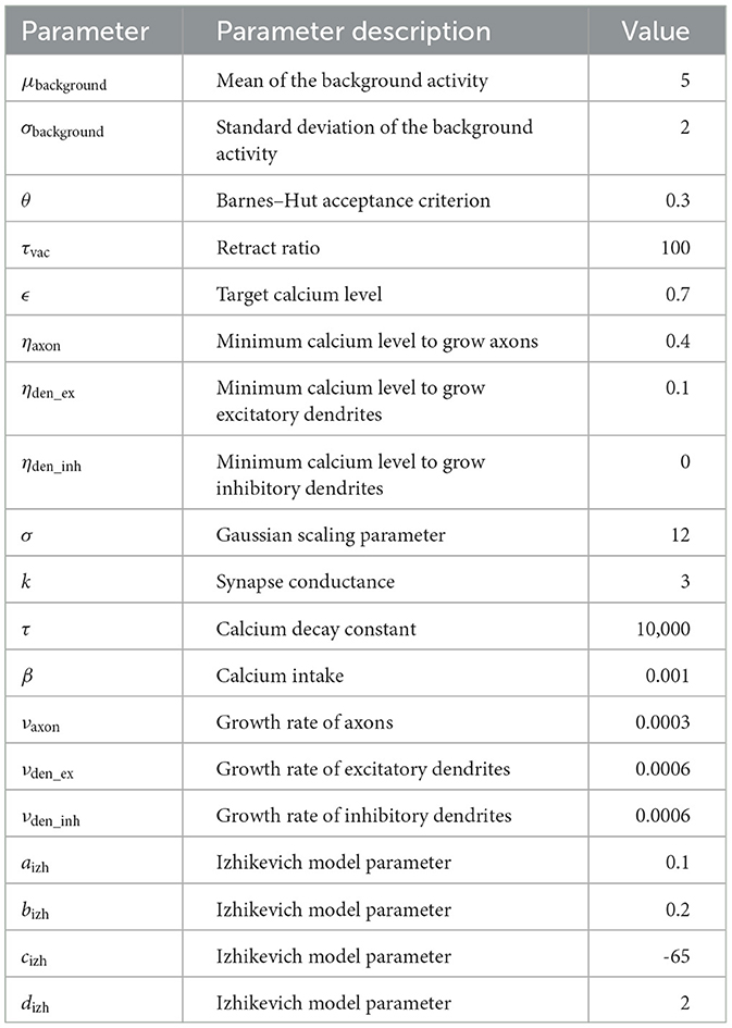
Table 1. Parameters for the experiments.

2.1.1 Growth model dCadt={−Caτ+βif neuron fires−Caτotherwise    (1)

The calcium concentration that acts as a proxy for the firing rate is described in Equation (1). It decreases over time with the time constant τ and increases by β when the neuron fires. Based on the calcium concentration, the number of synaptic elements of a neuron grows or shrinks as described in Equations (2–4). It depends on the growth rate ν, the current calcium concentration Ca, the minimum calcium concentration η required to grow synaptic elements, and the target calcium rate ϵ. Hence, if the calcium concentration is higher than the target, the neuron prunes synaptic elements; it grows new elements if the concentration is lower than the target. We follow Butz and van Ooyen (2013) for selecting our minimum calcium concentration ηaxon, ηden_ex, and ηden_inh, where they showed that a high ηaxon and a low ηden matches the experimental data and enables functional remapping.

dzdt=ν(2*exp(-(Ca-ξζ)2)-1)    (2) ζ=η-ϵ2-ln(0.5)    (4) 2.1.2 Forming and pruning of synapses

Since we already determined how many synaptic elements a neuron forms, we must now actually form synapses between unbound synaptic elements or prune them if the number of grown synaptic elements of a neuron is smaller than its actual synapses. In the last case, we chose a synapse to prune uniformly at random from all synapses of the neuron. Consequently, the synapse will be removed from the source and target neuron, independently of the number of grown synaptic elements of the partner neuron. When we need to form a new synapse, we search for vacant dendritic elements for every vacant axonal element. We choose a target element randomly based on weighted probabilities. Each target dendritic candidate is weighted with a probability based on the distance between the positions xi of the neuron of the inititaiting axonal element and the candidate's neuron position xj, as described in Equation (5). Note that the implementation uses an approximation (Rinke et al., 2018; Czappa et al., 2023) so that it does not need to calculate the probability for all candidates.

ki,j=exp(||xj-xi||22σ2)    (5)

Synaptic elements that are not connected are removed over time depending on the time constant τvac, as described in Equation (6).

dvacdt=-vacτvac    (6) 2.1.3 Electrical activity

The electrical input I is the sum of three inputs: synaptic, background, and stimulation, as described in Equation (7). The synaptic input Equation (8) is calculated over all fired input neurons j. Each of these synapses has a weight that of 1 for excitatory input neurons or −1 for inhibitory ones and is multiplied by the fixed synapse conductance k. The sum over those products for all input synapses of neuron j whose source neurons fired is the synaptic input for j. Additionally, the neurons are driven by a random, normally distributed background activity (Equation 9).

I=Isynaptic+Ibackground+Istimulation    (7) Isynaptic=∑jk*wj    (8) Ibackground~N(μ,σ2)    (9) 2.2 Izhikevich model

We chose the Izhikevich model (Izhikevich, 2004) as our neuron model because it enables modeling different spiking patterns and strikes a good compromise between biological accuracy and computational efficiency. We describe the membrane potential in Equation 10, where k0, k1, and k2 are constants and u is the membrane recovery variable as described in Equation 11. The membrane recovery depends on the fixed parameters a, b, and c and accounts for the hyperpolarization period of a neuron. Finally, we assumed that a neuron spikes if the membrane potential reaches 30mV. Then, we reset the membrane potential and membrane recovery variables according to Equation 12.

dvdt=k2v2+k1v+k0-u    (10) if v≥30mV,then{v←cu←u+d    (12) 2.3 Network setup and stimulation

Unless noted otherwise, our network consisted of 337,500 neurons, each with 20% inhibitory and 80% excitatory neurons. We distributed the neurons uniformly at random in a 3-dimensional cubic space. We split the network into 3 × 3 × 3 = 27 equally sized cubes with about 12,500 neurons each, following Gallinaro et al. (2022). In each box, we grouped a part of the neurons into disjoint ensembles of 333 excitatory neurons. We selected them randomly from all neurons in the box. Figure 1 visualizes the setup as a 2D example.

We started our network in a fully disconnected state and let it build up the connectivity from scratch for 1,000,000 steps. In more detail, the neurons received a normally distributed background activity such that they have a certain baseline activity. As this baseline is insufficient to reach the neurons' target calcium level, they grow synapses to connect to other neurons and receive more input. When the neurons reach the target calcium level, they stop growing synapses and they perform only small modifications to their synapses due to the fluctuations in the input noise and the resulting fluctuations in the neurons' firing rate. In this state, the network is in equilibrium, as every neuron is approximately at its target calcium level, and only small modifications are made to the network. We saved the newly formed network and used it as a starting point for our experiment. Hence, we continued the simulation with this network and waited for 150,000 steps until the network stabilized itself. Then, we continued the simulation with three stimulation phases similar to Gallinaro et al. (2022): baseline, encoding, and retrieval. We performed all stimulations for 2,000 steps with 20mV. In the baseline phase, we stimulated all US ensembles in step 150,000, followed by all C1 ensembles (250,000), and finally, all ensemble C2 (350,000). Note that US, C1, and C2 were stimulated after each other, but all ensembles of the same type across all boxes were stimulated at the same time. The goal of this phase is to strengthen the connectivity within each neuron ensemble. We selected the pause between the stimulation so that the neurons' calcium levels return to their target level to ensure that there is no priming effect. Moreover, the C2 ensemble acts as a control to counter a priming effect as well as we would see an effect not only in US and C1 but also in C2.

Then, in the encoding phase, we wanted to learn the relationship between US and C1 and, therefore, stimulated all US and C1 ensembles together in step 450,000 and all C2 ensembles in step 550,000. The stimulation of the C2 ensembles alone acts as a control against a priming effect. That would be the case when US or C1 form connections to C2 despite it being stimulated alone. Similar to the baseline phase, we stimulated the specified ensemble types from each box at the same time.

Later, in the retrieval phase, we turned the plasticity off so that no further modifications were possible. We did this to see how the network behaves without any further modifications. Here, we stimulated, beginning in step 650,000, all C1 ensembles consecutively in isolation, one after the other, with a pause of 18,000 steps between them. Note that this is different from the previous two phases, where we stimulated the same ensemble type (e.g., US) from each box at the same time. In the end, we stimulated all C2 ensembles together at step 1,190,000 as a control. We expect that the readout neuron of a box fires at an increased rate when we stimulate C1 of the same box due to the learned relationship and not if we stimulate the C2 ensembles. The protocol is visualized in Figure 2A.

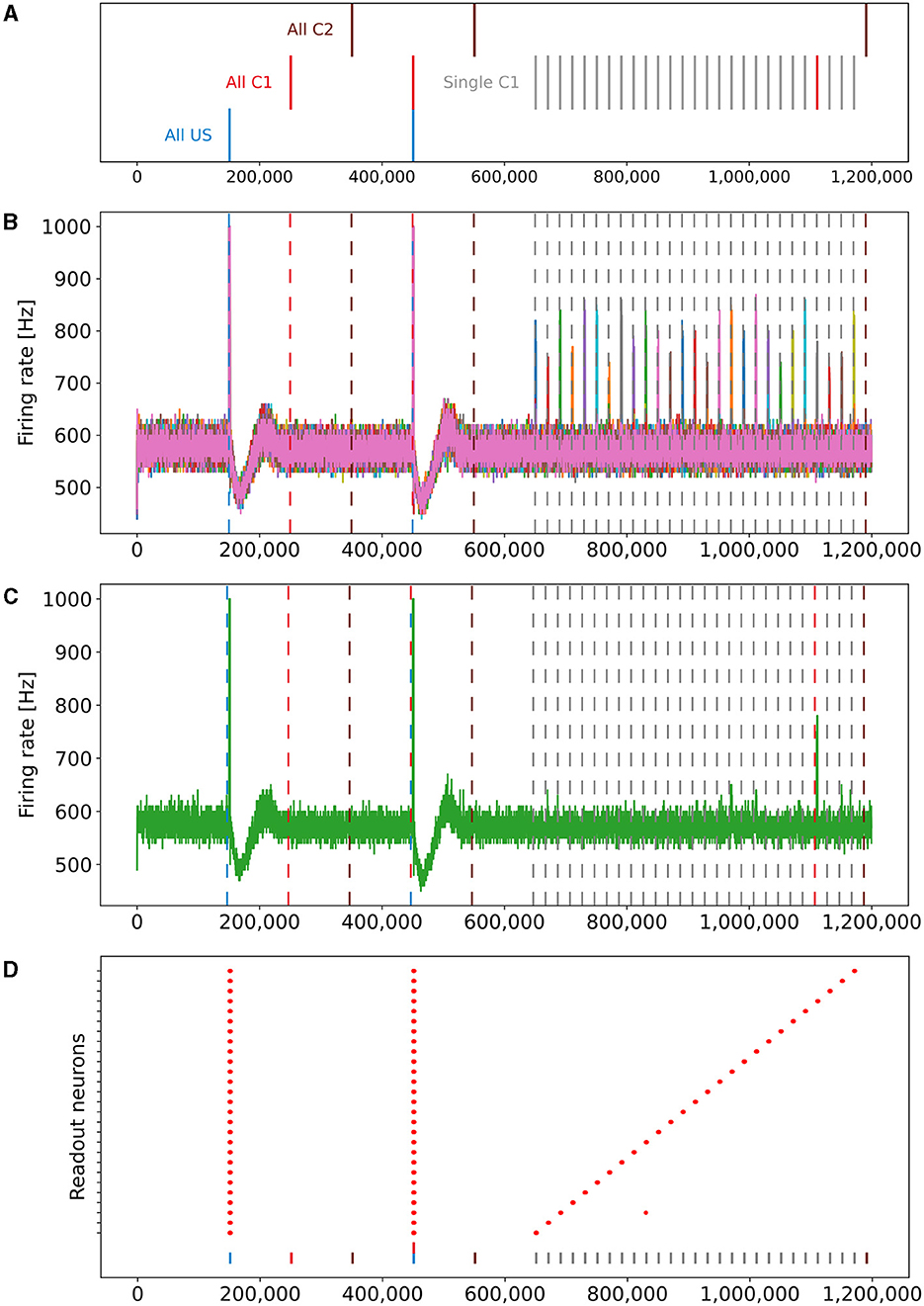
Figure 2. Stimulation protocol and firing rates (y-axis) of all readout neurons plotted over time (x-axis). The vertical dashed lines represent the stimulation of the ensembles US (blue), C1 (red), and C2 (brown). The gray lines and red line on the right represent single stimulations of C1. The readout neurons fire at an increased rate when US is stimulated in the baseline and encoding phase. If the model successfully learns the relationship between the ensembles US and C1 of the same box, neurons of ensemble US will also fire at an increased rate. (A) Stimulation protocol of the experiment. The experiment is split into three stimulation phases: baseline, encoding, and retrieval. (B) Firing rates of all 27 readout neurons laid over each other. (C) Firing rate of a single readout neuron. (D) Scatter plot when readout neurons fire at an increased rate. The 27 readout neurons are distributed along the y-axis. A red dot indicates that a readout neuron fires at an increased rate. The stimulation of all US (blue), C1 (red), C2 (brown), and single C1 ensembles (gray) are marked with a vertical bar at the bottom.

2.4 Validity check

To check the validity of our results, we needed to make an assumption about the distribution of the neurons' firing rate. We hypothesized that the firing rates follow a normal distribution and showed this with the Kolmogorov–Smirnov test. It calculates the probability that the distribution of our data is not the same as the given distribution to which we compare (in our case: normal distribution). For this, we simulated the network that resulted from our main experiment for 100,000 steps and recorded the times the readout neurons fire. Then, we split the steps into bins with the size of 1,000 steps and calculated the firing rate of each readout neuron for each bin. As we hypothesized a normal distribution, we calculated the mean and standard deviation for the calculated firing rates. The histogram of the firing rates is shown in Supplementary Figure 1. We applied the Kolmogorov–Smirnov test (Massey Jr, 1951) to the calculated firing rates and retrieved a p-value of 5.34*10−6. As a value of p smaller than 0.05 can be interpreted as non-significant, we can assume that our firing rates are normally distributed.

Now, we can continue with our validity check by checking the firing rate of the readout neuron during the retrieval phase to ensure that the network behaves as expected. We assumed that the firing rates follow a normal distribution and detect abnormal behavior of the readout neuron when its firing rate is significantly outside of the normal distribution. For it, we used the 3-σ rule (Pukelsheim, 1994), as described in Equation (13) with f as the firing rate of the readout neuron, μ as its mean, and σ its standard deviation without any stimulation. Approximately 99.7% of the normal firing rate lies within the interval of three times the standard deviation around the mean of the normal distribution of the firing rate. We considered a firing rate outside of this interval for at least 500 steps to be significantly different from the normal firing rate of the neuron when the network is in an uninfluenced state.

f∈[0,μ−3σ)              Significantly decreased firing ratef∈[μ−3σ,μ+3σ]                                   Normal firing ratef∈(μ+3σ,1000]        Significantly increased firing rate    (13)

We expected a readout neuron to fire at an increased rate if

• We stimulate its ensemble US during the baseline phase or,

• We stimulate its ensembles US and C1 during the encoding phase, or

• We stimulate its ensemble C1 during the retrieval phase.

It should not fire at an increased firing rate otherwise.

We allowed the increased firing rates to start (end) within 100ms of the start (end) of the associated stimulation to allow for some variation in the neurons' behavior.

2.5 Large-scale formation of memory engrams

We successfully repeated the experiment with a larger network to show how well our approach scales. Instead of 3 × 3 × 3 = 27 boxes, we split a larger network into 7 × 7 × 7 = 343 boxes with a total of 343·12, 500 = 4, 287, 500 neurons and stimulated the network following the same pattern as before. We analyzed the firing rates of the readout neurons to check whether they fired only when US was stimulated during the baseline and encoding phases and only when C1 in the same box was stimulated during the retrieval phase as described in Section 2.4.

2.6 Advanced simulations

The following two experiments started with the network that was stimulated as described in Section 2.3 because they analyze the newly created engrams.

2.6.1 Pattern completion

Gallinaro et al. (2022) showed that the stimulation of 50% of the neurons of a single engram was necessary to increase the activity of the rest of the engram; we will improve upon that in both the necessary threshold and the technical contribution. While we stimulated all neurons of ensemble C1 during the retrieval in the previous experiment, we now show that it is sufficient to stimulate only a subgroup of neurons in ensemble C1 to trigger the readout neuron in the associated ensemble US. Hence, after the previous learning experiment with 27 boxes, we continued simulating the network, picked a single ensemble C1 from one box, and stimulated varying numbers of neurons. To this end, we continued the simulation and waited for 60,000 steps until the network stabilized. Then, we turned the plasticity off and stimulated 5% randomly chosen neurons of the ensemble C1 of the center box for 2,000 steps. After a pause of 98,000 steps, we added a further 5% randomly chosen neurons of the ensemble to the stimulated neurons and stimulated them again. We repeated this cycle until we stimulated 100% of the ensemble.

2.6.2 Forming long-distance connections

During our main experiment, we wanted to build memory engrams only within a box. Now, we want to show that we can still form connections over long distances and therefore combine memory engrams from different regions. For this, we continued the simulation with a larger Gaussian scaling parameter σdistant that makes connections over long distances more probable. We selected two edge boxes on the opposite side of the simulation area to maximize the distance. We waited for 150,000 steps so that the network could stabilize first. Then, we stimulated the ensembles US and C1 from both boxes together for 2,000 steps. After a pause, we turned the plasticity off in step 250,000 and stimulated each ensemble C1 from the boxes after each other with a pause of 8,000 steps between them to check if the network learned the relationship between the ensembles in the two boxes without interfering with other boxes. As a last stimulation in the step 520,000, all of the ensembles C2 were stimulated to check the response to the control ensembles.

2.7 Ablation studies

We investigated how the network reacts to applied lesions. We are interested in two cases: The loss of synapses and the loss of neurons. For both cases, we continued the simulation from our main experiment and applied the lesion after 150,000 steps. Then, we waited 200,000 steps for the network to stabilize again so that each neuron reached its calcium level again. In step 350,000, we turned the plasticity off and stimulated all C1 ensembles after each other and all C2 ensembles as described for the retrieval phase in Section 2.3. We randomly selected a center of the lesion in each box and selected a fraction of neurons that are closest to this center. In step 150,000, we removed all connections from and to the selected neurons. If we decided to lesion the neurons, we also removed them from the network so they were not available for reconnecting their synapses.

3 Results

This section is divided into multiple parts. We will start with the analysis of the process of the formation of a single memory engram. Then, we will discuss the simultaneous formation of multiple memory engrams. Finally, we provide the results of the large-scale and advanced simulations.

3.1 Process of engram formation

Our experiment consists of three phases: baseline, encoding, and retrieval. We started with the baseline phase. As described in Section 2.3, the network was in a stable state with only minor changes in the connectivity at the beginning of the baseline phase (Figure 3) . At this point, the network's connectivity was random based on the neurons' distances (Figure 4B). This phase aims to form neuron ensembles with strong connectivity within the ensemble. The additional stimulations resulted in an increased firing rate (Figure 3A) of the neurons, which in consequence lead to an increase in their calcium level and therefore to a pruning of synapses (Figure 3B). After the stimulation ends, the firing rate fell before its usual level due to the smaller synaptic input caused by the pruning of synapses. Consequently, the neurons within the ensemble started regrowing their synapses until they reached a stable firing rate and calcium level as its target value. All neurons within the ensemble regrew their synapses simultaneously and are, therefore, looking for new synapse partners at the same time. This high ratio of potential partners within the same ensemble results in strong connectivity within this ensemble (Figure 3C). We stimulated a single ensemble, such as US, from each box at the same time. This and the property of forming new synapses based on the distance of neurons result in a strong within-connectivity of the ensemble in a box. After a short delay, we continued with the second C1 ensembles, after another delay with C2 ensembles. As a result, we had three strongly within-connected ensembles in each box representing an engram (Figure 4C). We refer to the study by Gallinaro et al. (2022) for details of this process. Figure 4 shows the process of reorganizing the connectivity during the entire experiment.

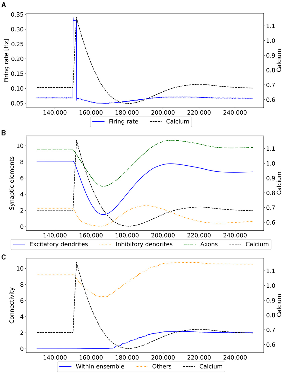
Figure 3. Mechanism of a single engram formation shown with a single ensemble group US. The stimulation in step 150,000 starts the engram formation. (A) Intracellular Calcium (right y-axis) as an indicator for the average firing rate (left y-axis) of all neurons in a randomly selected example US ensemble. The stimulation is visible as a high spike in the firing rate. This was followed by decreased activity caused by homeostatic network reorganization as depicted in (B, C). (B) Changes in intracellular calcium triggered growth of synaptic elements of the neurons in the exemplary ensemble. The synaptic elements decrease after the stimulation as calcium was higher than the homeostatic set-point and grew again afterwards when activities fell below the set-point as a consequence of compensatory pruning of synapses. (C) Average connectivity of an exemplary ensemble to itself and other neurons. As a consequence of the changing number of synaptic elements, we see a drop in the connectivity to neurons outside of the ensemble directly after the stimulation which was slowly restored afterwards. Connectivity within the ensemble increased likewise.

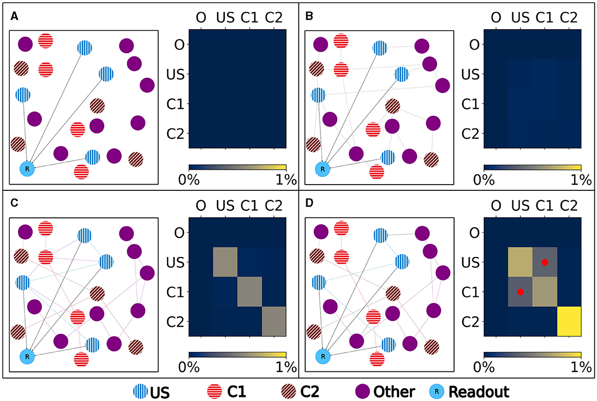
Figure 4. Left: Schematic illustration of the connectivity within a single box. Right: Heatmap of the neurons' normalized number of input (row) and output (column) connections of each ensemble (O), US, C1, and C2. Normalized with the size of the source and target ensemble.. (A) Visualization of the network at the beginning with no connectivity besides the static connections to the readout neuron. (B) Visualization of the network after the growth period with random connectivity. (C) Visualization of the network after the baseline phase with increased connectivity within each ensemble. (D) Visualization of the network after the encoding phase showing that the learned relationship between US and C1 is brought about by an additional increased connectivity between the ensembles C1 and US as marked in the heatmap with red dots.

Next, we continued with the encoding phase. In this phase, the model learned the association between the memory ensembles US and C1 within each box. For this, we stimulated the ensembles US and C1 together. Consequently, the ensembles US and C1 in a single box form many connections using the same mechanism as in the baseline phase (Figure 4D).

Finally, in the retrieval phase, we checked if the model learned the association between US and C1. The firing rate of an exemplary single box's readout neuron is visualized in Figure 2C. In addition to the two spikes during the earlier phases when US was stimulated, the readout neuron fired only at an increased rate when the ensemble C1 from the same box was stimulated and not if we stimulated our control ensemble C2 or any other ensemble from another box.

3.2 Simultaneous formation of memory engrams

Our network consisted of 3 × 3 × 3 = 27 boxes, each with three ensembles: US, C1, and C2. By plotting the readout neurons in Figures 2B, D, we show that the network learns the relationships between US and C1 in each box and not between US and C2. Without stimulation, the readout neurons fired at about 600Hz. All readout neurons fired at steps 150,000 and 450,000 with the maximal frequency of 1000Hz. This was followed by a decrease of the firing rate to about 450Hz until it recovers to its normal frequency of 600Hz. In step 150,000, we stimulated the US ensembles directly connected to their readout neurons during the baseline phase. During the stimulations of C1 in step 250,000 and C2 in step 350,000, the readout neurons did not fire at an increased rate compared to their baseline frequency. This shows that the network works as desired because the unconditioned reaction is shown after the unconditioned stimulus. Later, during the encoding phase, the readout neurons fired again, as expected when US and C1 were stimulated together in step 450,000 but not when C2 was stimulated in step 550,000. Finally, in the retrieval phase, we stimulated the ensemble C1 from each box after each other. The readout neuron of the same box fired when its ensemble C1 was stimulated, indicating that the network learned the relationship between US and C1 only within the same box but not beyond box boundaries. The firing rates were lower than during the stimulation in the encoding phase but still very distinguishable from the rest of the activity. We noticed small spikes of some readout neurons when another box was stimulated. However, the stimulation of our control ensembles C2 still did not influence the readout neurons.

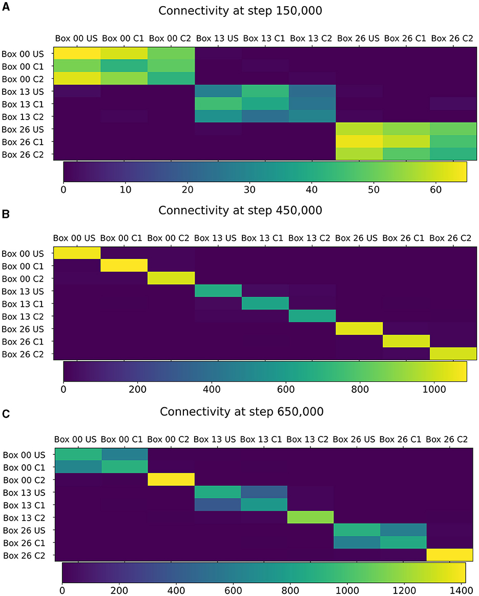
The learned relationship between US and C1 in each box can be explained with the newly formed connections, as visualized in Figure 5. At the beginning of the simulation, all ensembles were randomly connected (Figure 5A). After the baseline phase, the connectivity within the ensembles increased, and the connectivity between different ensembles decreased (Figure 5B). This increased connectivity within ensembles indicates the formation of memory engrams similar to Gallinaro et al. (2022). However, in contrast to what they did, we stimulated all US and C1 ensembles together only once instead of thrice. After the encoding phase, the connectivity between the ensembles US and C1 in the same box increases significantly, clarifying that the network learned the relationship between US and C1 (Figure 5C). However, we could observe a slightly increased connectivity between the ensembles of neighboring boxes due to the connectivity probability being based on the distance of neurons. This explains the slightly increased activity of the readout neurons sometimes when another box is stimulated. Furthermore, the C2 ensembles formed connections primarly within their ensembles and did not connect to neurons in other boxes or ensembles, confirming that these control ensembles did not influence the learning process.

Figure 5. Connectivity between chosen ensembles in the network. From the top left box of the first layer (box 00) over the center box of the second layer (box 13) to the bottom right box of the last layer (box 26). (A) During baseline phase, before first stimulation at step 150,000, connectivity is randomly distributed but predominantly remains within a box. (B) After baseline phase at step 450,000, connectivity has increased within each neuron ensembles. (C) After the encoding phase at step 650,000, connectivity also increased between ensembles US and C1 within the same box.

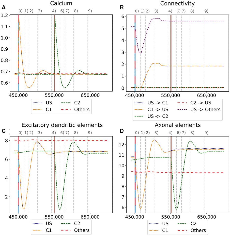
3.3 Spatiotemporal dynamics of homeostatic engram formation

We observe the average calcium level, grown axons and excitatory dendrites, and the connectivity of the neurons over the entire reorganization process for the ensembles US, C1, and C2 for an exemplary single box in Figure 6 to analyze the mechanism behind the synaptic reorganization further. Moreover, we visualize the average calcium level and, therefore, indirectly, the activity of the neuron groups at different times in the context of the growth curves for the different types of synaptic elements in Figure 7A. Before the first stimulation in the encoding phase of the ensembles US and C1, the calcium level of all groups was around their target level (Figure 7A left). The values of the growth curves for this activity level were at around zero as the model is in an equilibrium state with only minor modifications to the network, which is also visible in the almost constant number of axons and dendrites, as illustrated in Figures 6C, D. The connectivity between US and C1 was almost zero, as there is no relationship between them yet. Instead, the connectivity from within the ensemble US to external neurons was only high for neurons outside of any ensemble just because of the higher number of neurons not belonging to an ensemble compared to the size of the ensembles C1 and C2. Next, we applied the stimulation to the US and C1 ensembles (Figure 6 (0)), causing their activity to increase and moving the calcium for these ensembles to the right in Figure 7A (center). The values of the ensembles' growth curves were almost -1 for this calcium level, reducing the synaptic elements at maximum speed. Consequently, the number of axons and dendrites and their connectivity started decreasing.

Figure 6. Homeostatic reorganization of neuron ensembles within a single box during the encoding phase. All graphs are averaged over all neurons of the respective ensemble within a single box. We stimulated the ensembles US and C1 at step 450,000 (vertical red-blue line) and the ensemble C2 at step 550,000 (vertical brown line). Panels show the average intracellular calcium concentration (A), connectivity (B), amounts of excitatory dendritic elements (C) and axonal elements (D). Networks are in a homeostatic equilibrium before first stimulation (0). After stimulation, activity of the ensembles US and C1 is increased, resulting in pruning of synapses until calcium levels fall below the target value (1). Then, synaptic elements are formed, and calcium level may rise again (2). Axonal and dendritic elements are simultaneously formed by neurons of ensembles US and C1, which become available for synapse formation and explain the observed connectivity increase between these ensembles. The growth phase is followed by a transient overshoot (3) and subsequent minor pruning until a homeostatic equilibirum is reached again (4). The stimulation of C2 (5) follows the same trend [(5)-(9)] with the main difference that neurons from ensemble C2 are the only ones that grow axonal and dendritic elements at the same time. The consequence is a massive increase of connections within the ensemble but not between C2 and ensemble US.

Figure 7. The average calcium level of groups of neurons of a single box (x-axis) with calcium-dependent growth curves (y-axis). (A) Calcium level before and after the ensembles US and C1 were stimulated at step 450,000. Subsequentially, their calcium levels increased and growth curves caused synaptic elements to decrease and synapses to prune. When stimulation stopped and synapses were pruned, activities and calcium levels, respectively, dropped below the homeostatic set-point which, in turn, triggered the growth of synaptic elements and potentially also the growth of new synapses. Note, that calcium levels below the set-point were in an optimal regime for axonal element formation while dendritic elements grew slower. A surplus of axonal elements may result in more long-range connections while a prolongued growth of dendritic elements extended the phase in which new engrams could form because it may take longer until activities return to a homeostatic set-point. (B) Average calcium levels during ablation studies in which we removed connectivity of 50% of the neurons in a box. Directly after the stimulation, calcium levels of lesioned neurons dropped due to the lack of input. As a result, the neurons start regrowing synaptic elements until enough synapses were formed to restore activity homeostasis. The homeostatic reorganization is comparable to engram formation after stimulation in A. Note, that even for higher deletion rates neurons will return average firing rates to the homeostatic set-point (data not shown) very much as in (B), however without functional recovery of trained engrams.

After the stimulation ended, the calcium levels fell below their target (Figure 6 (1)). The neurons started rebuilding their synapses as soon as the calcium level dropped below its target level. The decrease in the calcium level was slowed down until it reached its lowest level (Figure 7A right, Figure 6 (2)). At this calcium level, the ensembles US and C1 correspond to the spike of the growth curve of the axons. The growth curves of the dendrites are lower but still positive. Hence, the ensembles US and C1 build new synapses fast, as shown in Figures 6C, D. As the ensembles US and C1 built new synapses simultaneously, they formed their synapses to a large degree between themselves, increasing connectivity between them (Figure 6B). The fast formation of synapses caused the calcium level to exceed its target (Figure 6 (3)) due to the increased synaptic input and, therefore, led again to a slight reduction of synaptic elements. In the end, the calcium levels of all groups returned to their set level (Figure 7A bottom, Figure 6 (4)) and the connectivity as well as the number of synaptic elements remained at a stable level. During the entire stimulation and reorganization of the ensembles US and C1, the calcium level, number of synaptic elements, and connectivity of the control ensemble C2 remained unchanged. The reaction of the ensemble C2 followed the same trend as the ensembles US and C1 during and after its stimulation (Figure 6 (5)-(9)). As we stimulate the ensemble C2 on its own, we see no effect on the other ensembles.

When we look at the course of the calcium levels before (Figure 7B left) and after (Figure 7B center) we removed all connectivity between a group of neurons (Figure 7B), we observe that the levels dropped from their target level for the lesioned group of neurons. The decreased calcium level corresponds almost to the peak of the growth curve for axons (Figure 7B center), meaning that axons were built at their maximum speed. Moreover, dendrites were also built fast but not at their maximum speed. As a result of the build-up of synaptic elements, the activity and, therefore, the calcium levels of the lesioned neurons started increasing until they reached their target level again (Figure 7B right). The calcium level of the non-lesioned neurons remained mostly unchanged. The rebuilding of the synaptic elements after completely removing them for the lesioned neurons is similar to rebuilding the synapses after the stimulation during the conditioned learning experiment. This explains why the network can only recover its learned relationships if all or a high ratio of the lesioned neurons are part of the learned relationship. Otherwise, the network expresses the same learning effect as before but between all lesioned neurons regardless of the affiliation of the neurons.

As we could observe, the synaptic reorganization in our model always follows the same pattern. First, there is a loss of connectivity either directly caused by a lesion or indirectly caused by stimulation and the following pruning of synaptic elements caused by the increased activity and the growth rule of our model itself (Figure 6 (0)-(1)). In consequence, the activity of the neurons decreases because of the smaller synaptic input. Then, neurons start rebuilding the synapses, connecting mostly among themselves (Figure 6 (1)-(4)). In the end, the activity of the neurons returns to its initial level. This contrasts Hebbian plasticity, where we cannot observe such a sequence of events. Neurons with similar activity patterns, e.g., because of stimulation, directly strengthen their connections. Strengthening their connections makes it more likely that they fire together and increase their activity. As they are now more likely to fire together, Hebbian plasticity continues to strengthen their synapses. This can lead to continuous strengthening of synapses and increasing neuron activities with unbound synaptic weights. Multiple counter mechanisms have been discussed (Chen et al., 2013; Chistiakova et al., 2015; Fox and Stryker, 2017) to counter the runaway activity of Hebbian plasticity. Integrating our model of structural homeostatic plasticity with Hebbian plasticity could also counter this problem. While most models are difficult to observe in experiments, our model shows an observable sequence of events during learning that could be tested in experiments.