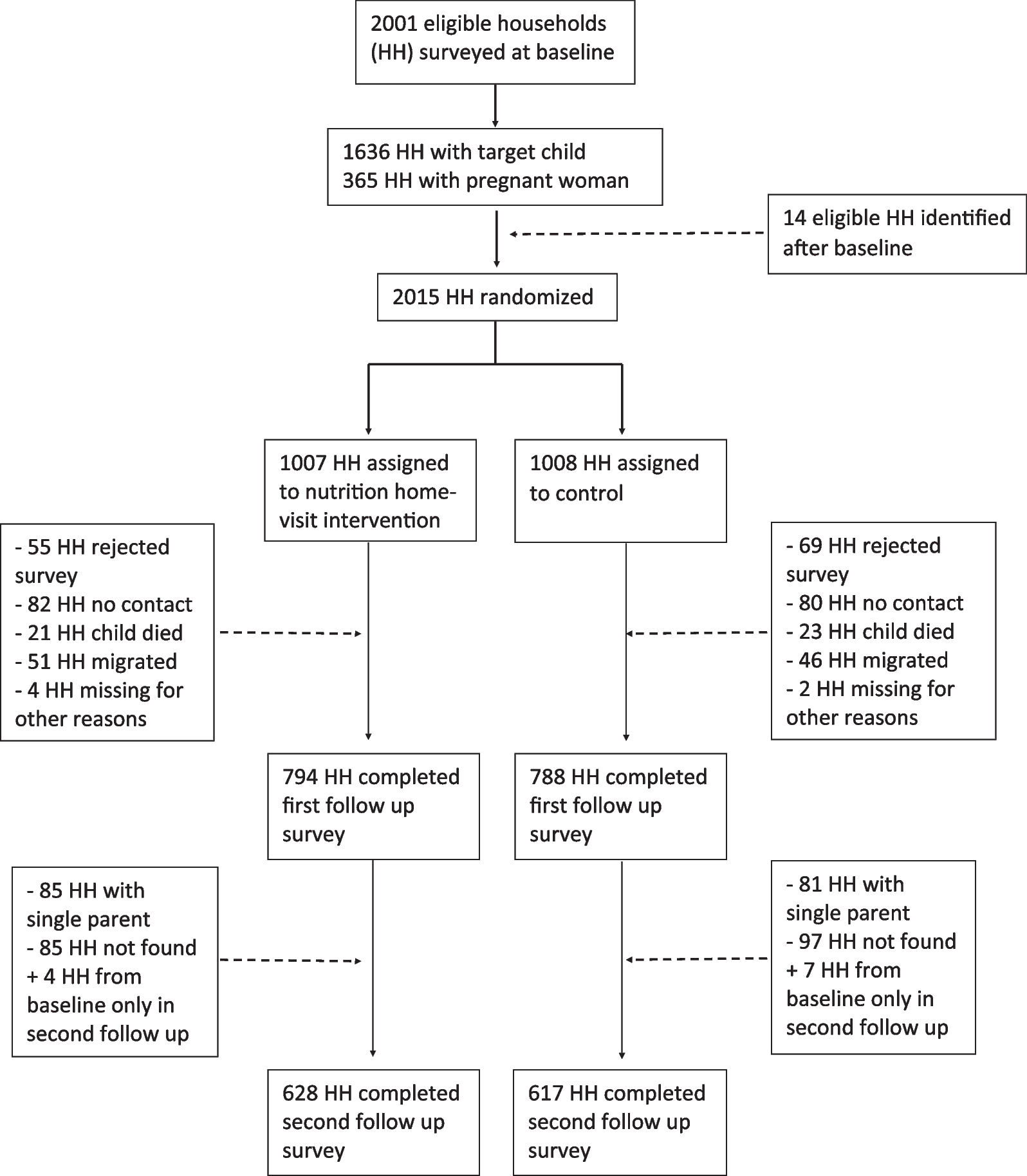
The study uses secondary data from the 2015/16 Malawi’s Demographic Health Survey (MDHS) as part of national surveys implemented by the National Statistical Office for Malawi over a 4-month period, from 19 October 2015 through 17 February 2016. The sampling frame used for the 2015/16 MDHS was the frame of the Malawi Population and Housing Census (MPHC), conducted in Malawi in 2008. The 2015/16 MDHS sample was stratified and selected in two stages. Each district was stratified into urban and rural areas. In the first stage, 850 standard enumeration areas (SEAs), including 173 SEAs in urban areas and 677 in rural areas, were selected with probability proportional to the SEA size and with independent selection in each sampling stratum. In the second stage of selection, a fixed number of 30 households per urban cluster and 33 per rural cluster were selected with an equal probability systematic selection from the newly created household listing. A total of approximately 24,562 women were interviewed. The Woman’s Questionnaire collected information from eligible women age 15–49 who were asked different sets of questions. Of interest for this study was background characteristics; Reproduction: children ever born, birth history; Maternal and child health, breastfeeding, and nutrition: prenatal care, delivery, postnatal care, breastfeeding and complementary feeding practices, vaccination coverage.

A total of 17,286 live birth were recorded over a five-year recall period preceding the survey and these were the candidate cases for infant mortality analyses. The women questionnaire included questions on whether the women had ever born a child and the current age of the child. This information was used to subset the data of children born within the last 5 years prior to the survey. The children included for analysis were those born between 2010 to 2015 for the women interviewed in 2015, and between 2011 to 2016 for those women interviewed in 2016.

Variables: The outcome variable in this study was time to death of an under-five child. Death happening between anytime from birth to 59 months was considered as an event. Children surviving 59 months were censored. Death was not characterized, regardless of any cause, any occurrence of death for the under-five child was considered an event. A number of covariates were introduced to control for drivers of deaths. Building on the previous studies as earlier reviewed this study included the following covariates: Mothers age, Mother’s education level, Wealth Index, Sleeping in treated net, Breastfeeding, Place of birth, Birth weight of the child, antenatal visits.

To provide contextual understanding of the variables included in the analysis, a univariate analysis was conducted on the socioeconomic, demographic factors and child survival. Chi-square test of independence was used to test bivariate relationship between covariates and survival/failure outcomes. Child survival was estimated using:

$$_=\prod_1-\frac_}_}$$

(1)

where ti is duration of a child at any point of the 59 months period, dt is mortality event up to point t, nt is the number of children that are at risk of mortality spell just before ti. [6].

The cox-proportion hazard model was used for multivariate analysis. The cox models determine the probability of event happening over a given interval which is given as the ratio of survival or hazard probabilities. It reflects the length of time a child survived before dying. The inclusion of covariates necessitates computation of how often death occurs in one group compared to the reference group [12]. The Cox proportional hazards model was fitted as follows:

$$\lambda \left(t|x\right)=_\left(t\right)}(\beta x)$$

(2)

where \(\lambda \left(t|x\right)\) is the hazard function for the child living up to less than 59 months. The hazard is a function of some unspecified “baseline hazard \(_\left(t\right)\) and a set of covariates defined by X, \(\beta\) is a coefficient vector for various covariates included in the model. The covariates act to multiply the baseline hazard in a time-independent manner [3]. From this model, we derive the hazard ratios. The time-varying coefficient was fitted by extending above basic model as:

$$\lambda \left(t|z(t)\right)=_\left(t\right)}(\beta x+\gamma Xg(t))$$

(3)

where \(\beta\) and \(\gamma\) are coefficients of time-fixed and time-varying covariates, respectively [26]. To model heterogeneity, shared frailty model was fitted. A frailty model includes, in the hazard function, the value of an additional unmeasured covariate, the frailty, denoted by \(\gamma\), yielding a hazard function as using:

$$_(t)=_\left(t\right)}(\beta _+_)$$

(4)

where \(_\left(t\right)\) is the hazard function for the jth individual belonging to i th cluster, \(_\left(t\right)\) is the baseline hazard at time t, \(_\) is the vector of k covariates and \(_\) is the random effect for the ith cluster [14]. We assume that that the frailty is independent of any censoring that may take place. Because the hazard cannot be negative, distributions must have only positive values. This and other technical issues have led, most frequently, to the use of the Gamma distribution (i.e., a model that assumes that the frailties represent a sample from a Gamma distribution with mean equal to 1 and variance parameter 9). To avoid imposing inappropriate distribution on the frailty, we test it under gamma and inverse-gamma distribution and select the one that is more suited to the data based on smallest Akaike Information Criterion values. Similarly, the baseline hazard can assume various distributions. Hence, in our specification we test the baseline hazard under several distributions including Exponential, Weibull, Loglogistic, Lognormal, Gompertz, Exponential, Weibull, Loglogistic, Lognormal, Gompertz. We also select the model with the smallest Akaike Information Criterion value.

The parameter \(\beta\) is found by maximizing the partial likelihood. In order to formulate the partial likelihood, the f unique failure times are ordered increasingly \(_\) < ··· < \(_\) and j(i) is the index of the sample failing at time ti. Let \(}_}\) be the row vector of covariates for the time interval (\(_\); \(_\)] for the ith observation in the dataset i = 1, …, N. We use a method that obtains parameter estimates, \(\widehat\), by maximizing the partial log-likelihood function for the Cox model:

$$}\mathcal(\beta )=\sum_^\left[\sum_\beta \top _-_}\left\_}}\left(\beta \top _\right)\right\}\right]$$

(5)

where j indexes the ordered death times t(j), j = 1,..., D; Dj is the set of dj observations that fail at t(j); dj is the number of failures at t(j); and Rj is the set of children k that are at risk at time t(j) (that is, all k such that t0k < t(j) ≤ tk). This formula for \(}\mathcal(\beta )\) is for unweighted data and handles ties by using the Peto–Breslow approximation [2, 16], which is the default method of handling ties. The method treats efficient score residuals as analogs to the log-likelihood scores one would find in fully parametric models. Tied values are handled using Breslow approach as:

$$}_=\sum _^\sum __}\left[}_\left(_\beta +}}_}}\right)-}_}\left\_}}_l }(xl \beta }}_}})\right\}\right]$$

(6)

where wi are the weights. In the log likelihood for the Breslow method, \(}_=_\times N/\sum _\) when the model is fit using probability weights, and \(}_=_\) when the model is fit using frequency weights or importance weights. Calculations for the exact marginal log likelihood (and associated derivatives) are obtained with 15-point Gauss–Laguerre quadrature. The method provides approximation of the exact marginal log likelihood. While the Efron approximation is a better (closer) approximation, but the Breslow approximation is faster.

For shared-frailty models, the data are organized into G groups with the ith group consisting of ni observations, i = 1, …, G. From Therneau and Grambsch [20], estimation of \(\theta\) takes place via maximum profile log likelihood. For fixed\(\theta\), estimates of \(\beta\) and ν1, …, νG are obtained by maximizing

$$\begin & \log L\left( \theta \right) = \log L_ \left( , \ldots , v_ } \right) \\ & \quad + \mathop \sum \limits_^ \left[ \left\ - \exp \left( } \right)} \right\} + } \right.\left( + D_ } \right)\left\ + D_ } \right)} \right\} - \frac + \left. \left( + D_ } \right) - \log \left( } \right)} \right] \\ \end$$

(7)

where Di is the number of death events in group i, and logLCox(\(\beta\); ν1, …, νG) is the standard Cox partial log likelihood, with the νi treated as the coefficients of indicator variables identifying the groups. That is, the jth observation in the ith group has log relative hazard \(x\beta\) + νi. The estimate of the frailty parameter, \(\widehat\), is chosen as that which maximizes logL(\(\theta\)). The final estimates of \(}\) are obtained by maximizing logL(\(\widehat\)) in \(}\) and the \(_\).

The estimated variance–covariance matrix of \(\widehat}}\) is obtained as the appropriate submatrix of the variance matrix of (\(\widehat}}\), \(}}}_,\boldsymbol\dots ,}}}_}}\boldsymbol)}_\) and that matrix is obtained as the inverse of the negative Hessian of logL(\(\widehat}}\)). Therefore, standard errors and inference based on \(\widehat}}\) should be treated as conditional on\(\theta = \widehat}}\).

The likelihood-ratio test statistic for testing H0: θ = 0 is calculated as minus twice the difference between the log likelihood for a Cox model without shared frailty and logL(\(\widehat}}\)) evaluated at the final (\(\widehat}}\),\(}}}_,\boldsymbol\dots ,}}}_}}\boldsymbol)}_\).

The DHS surveys are designed using a complex survey design that involves stratification, clustering, and weighting to ensure that the survey sample is representative of the population of interest. Frailty models can account for clustering by including a random effect or frailty term in the model that captures the unobserved heterogeneity between the clusters.

Ethics approval was not required for this study since the data is secondary and is available in the public domain. More details regarding MDHS data and ethical standards are available at: http://goo.gl/ny8T6X