The simplified wings used in this study are identical to the wings previously used in numerical (Engels et al. 2021) and experimental approaches (O’Callaghan et al. 2022). Wing design and kinematic pattern are explained in great detail in the latter manuscripts, and we thus refer to the materials and methods section of both studies for further information. Here, we only present a short description of the experimental approach. The snow cone-like model wings were printed from polyvinylalcohol plastic (PVA) using a high-resolution Ultimaker3 3D printer (Ultimaker, Utrecht, the Netherlands) with Cura 4.8 software. The wings had a narrow root, different number of bristles with varying spacing (Δb), attachment sites and area coverage (Fig. 1d, e). We defined bristle spacing Δb as the mean distance between two bristle tips of natural wings but excluded 20% of the smallest and largest bristles. We tested wings with a ∆b (number of bristles) of 0.163 (9), 0.109 (14), 0.081 (19), 0.065 (24), 0.054 (29), 0.033 (49), 0.022 (74), 0.016 (99) and 0 (fully membranous, Fig. 2d). These values are equal to a relative covered area of approximately 0.21, 0.23, 0.24, 0.26, 0.28, 0.34, 0.42, 0.51 and 1.0, respectively (O’Callaghan et al. 2022). The wing shaft covers ~ 20% area of the fully membranous wing. Wing thickness was ~ 2.0 mm at the base and ~ 1.3 mm at the end of the membranous core. Bristle diameter was ~ 1.1 mm or ~ 8.8 \(\times\) 10–3 wing length and bristle orientation relative to the wing's longitudinal axis was ~ 29° (Fig. 1e). The wing with Δb = 0.016 was similar to the natural archetype of Gynaikothrips ficorum that has 173 bristles, a bristle angle of 54.9°, a bristle spacing of 0.0125R, and 0.101R bristle length (wing length, R; Fig. 1c, d). In the thrip, wingbeat frequency is 196 Hz and Reynolds number Re = 24 (see below for Re of model wings). The 3d-printed bristles were made rather rigid, because real wing bristles are remarkably stiff (Jiang et al. 2022) and a theoretical model predicts only negligible bristle bending during wing flapping motion (Engels et al. 2021). The wings were flat, because the contribution of wing corrugation to net aerodynamic forces is minimal in insect wings (Engels et al. 2020).

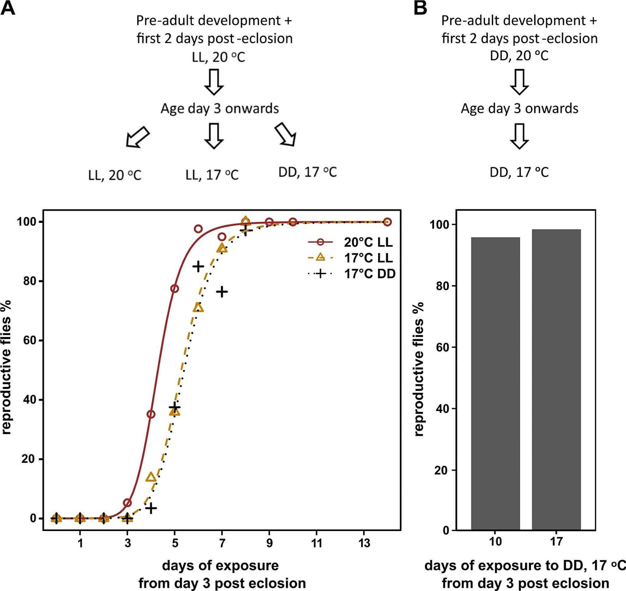
Experimental setup, wing kinematics and tested wings. a Wing models are flapped by two servo motors for horizontal flapping and wing rotation. The wings were immersed in a 60 × 40 × 36 cm3 tank filled with glycerine and flapped ~ 6 cm below the fluid surface to avoid wave generation. A turning stage allows manual rotation of the flapper and orientation of the wing towards the camera for particle image velocimetry (PIV). The tank is seeded with small air bubbles. b A generic lift-based kinematic with the wing's feathering angle (red), horizontal flapping angle (blue), and vertical heaving angle (green). c Lollipop diagram of a wing chord in xy-space with markers indicating the leading edge of the wing. The different times of the stroke cycle are colour-coded. d Cartoons of the tested solid (membranous) and bristled wings

For testing, the wings were immersed in a flow tank (~ 60 cm width, ~ 36 cm height, and ~ 40 cm depth) filled with glycerine (density, ~ 1260 kg m−3) and flapped by two small commercial servo motors (Graupner DS-series, Graupner, Germany) and a timing belt (Fig. 2a). The motors were position-controlled by an ATmega16L micro-controller on a STK500 board (Microchip AVR, Chandler, Arizona, USA). Motors and wing mechanics were mounted to a laser-calibrated turning stage that let us position the wing’s reference position at arbitrary angles towards the camera. This allowed us to map the wake throughout the entire stroke cycle. Each wing flapping sequence consisted of 10 consecutive stroke cycles with ~ 15 s resting periods in between, allowing the fluid to settle. The model wings flapped back and forth around the root in the horizontal direction with constant velocity and at 150° amplitude. Stroke cycle time was 3.876 s. The timing of wing rotation at the stroke reversals was symmetrical each lasting ± 10% cycle time (Fig. 2b, c). The wing’s feathering angle was 45° during the up and down strokes and 0° (vertical position) at the stroke reversals. Mean Reynolds number based on wing length and wing tip velocity was ~ 3.4 in all experiments (Engels et al. 2021; O’Callaghan et al. 2022) and fluid temperature ~ 24 °C.

To visualize vortices at the wing and in the wake, we seeded the glycerine by pumping air through a metal filter. The seeding consisted of small air bubbles with low mean upward velocity (~ 0.3 mm s−1) and high concentration. To minimize measurement errors associated with upward-drifting air bubbles, we waited approximately 1 h after seeding before starting flow visualization, allowing larger bubbles to disappear. The air bubbles were illuminated by a 50 mJ per pulse dual mini-Nd:YAG laser (Insight v. 5.1, TSI, USA) that created two identical positioned light sheets with ~ 3 mm thickness. Laser optics consisted of 1000 mm concave, –25 mm cylinder and –15 mm cylinder lenses. The timing between two laser pulses (∆t) varied depending on where the light sheet intersected with the wing to achieve 50% local overlap between the two PIV images, ranging from 9520 µs at the wing tip to 23,730 µs at the wing section nearest the root. The orientation of the light sheets was always perpendicular to the wing's longitudinal axis. For mapping the flow throughout the entire stroke cycle, we also used two self-built external delay circuitries that allowed us to trigger the laser pulses with various delays with respect to the onset of each flapping cycle.

The three-dimensionally printed PVA is not transparent. Wake and air bubbles on one side of the wing were thus shadowed, producing several missing fluid vectors during PIV analysis. Instead of combining PIV vectors of the two half strokes, we solved this problem using tilted mirrors (tilting angle 10–15°, Fig. 2a) behind the wing. These mirrors reflected the laser light that passed the wing above and below the stroke plane back into the PIV light sheet, allowing flow quantification of the entire fluid around the wing. Paired images of a 170 × 170 mm2 flow field were captured using a PowerView 2M camera equipped with a 50 mm lens (aperture 11, Nikkor AF, Nikon) and a green filter to reduce reflections from the ambient light. Data processing involved a two-frame cross-correlation of pixel intensity with a recursive Nyquist grid and a Hart correlator engine with bilinear peak engine. The interrogation area was 32 × 32 image pixels that resulted in 6,825 vectors per image. Vectors exceeding a tolerance of 6-times standard deviations were removed from the data set. We applied a neighbourhood mean filter with a tolerance of 2.0 ms−1 to the vectors and missing vectors were interpolated. At final post-processing, we applied a moderate smoothing algorithm with a neighbourhood size of 5 × 5 vectors and a Gaussian radius of 1.1.

To remove the flow component due to the wing's own flapping motion in the horizontal, we estimated the horizontal velocity for each wing section and subtracted this velocity component from all fluid vectors in the image. Some of the graphs in this study thus show the flow as the wing (animal) experiences the fluid and not the velocity that is seen by the observer outside the flow tank. As a consequence, the magnitude of velocity vectors near the wing is close to zero. Velocity subtraction and vorticity calculations were done by a TSI plug-in macro for Tecplot 9.0 (Tecplot, Inc., USA). To estimate mean fluid velocity, peak vorticity and circulation of vortical structures in a region-of-interest, we used a self-written software macro in Origin 7.0 (Microcal Origin, Inc, USA).

Although the flow during wing flapping is three-dimensional, fluid velocities in the spanwise direction of the wing (axial flow) were thought to be negligible because of low Reynolds number. This assumption is supported by detailed experimental and numerical analyses on the loss of enstrophy of the LEV in Drosophila model wings (see supplemental material in Lehmann et al. 2021). The latter study found that axial flow and vortex stretching are minimal during wing flapping, compared to other flow components. The study thus implied that two-dimensional measurements are sufficient to characterize the temporal development of vorticity. Remarkably, these data are valid for a Reynolds number 63-times higher than the one used in this study (~ 214 vs. ~ 3.4). At a Reynolds number of ~ 3.4, a 2-dimensional analysis of vorticity should thus be more than sufficient to estimate vortex strength during wing flapping. We averaged the measurements from the 3rd to the 8th stroke cycle (N = 6 cycles) because vorticity and forces are slightly higher in the first two stroke cycles after starting wing flapping from rest (O’Callaghan et al. 2022). If not stated otherwise, all presented data are means ± standard deviation.