Introduction

Spinocerebellar ataxia type 3 (SCA3), also called Machado–Joseph disease (MJD), is a common polyglutamine (polyQ) disease. PolyQ diseases are neurodegenerative disorders, and include Huntington's disease (HD), spinal bulbar muscular atrophy (SBMA), dentatorubral pallidoluysian atrophy (DRPLA), and spinocerebellar ataxia (SCA) types 1, 2, 3, 6, 7, and 17. The age at onset (AAO) of polyQ diseases is usually at middle age, and after that, the condition progressively worsens for 10–30 years until death (Ross, 1997; Fan et al., 2014). Although many studies have focused on the treatment of polyQ disease, there is no effective clinical treatment (Esteves et al., 2017; Paulson et al., 2017; Coarelli et al., 2018; Brooker et al., 2021; Costa and Maciel, 2022). Current treatments can only alleviate the symptoms and delay the progression of the disease after onset, and the treatment goals are to improve the motor performance and the quality of life (Ashizawa et al., 2018; Rodríguez-Díaz et al., 2018; Klockgether et al., 2019; Lanza et al., 2020). However, patients with mild symptoms are more likely to benefit from treatment (Miyai et al., 2012). Animal experiments also show that some potential treatments may prevent or reverse the progression of the disease, but they are more suitable for the early stage (Ashizawa et al., 2018; Friedrich et al., 2018). Therefore, AAO prediction contributes to early initiation to slow the progression and helps health care and social security agencies provide follow-up visits to improve the treatment efficacy (Jacobi et al., 2015; Paulson et al., 2017).

PolyQ diseases are caused by expanded cytosine-adenine-guanine (CAG) trinucleotide repeats. The relationship between the expanded CAG repeat (CAGexp) length and the AAO of polyQ diseases has been proven, and the AAO decreased with increasing CAGexp length (Collin et al., 1993; Gusella and Macdonald, 2000; Tang et al., 2000; Chattopadhyay et al., 2003; França Jr et al., 2012; Tezenas Du Montcel et al., 2014). However, the relationship between the AAO and modified genes is complex. The CAG repeat length of the expanded ATXN3 is the major AAO factor of SCA3/MJD, but other polyQ-related genes (CACNA1A, TBP, KCN3, RAI1, HTT, ATN 1, ATXN1, 2, and 7) and gene interactions also have modifying effects on the AAO (Andresen et al., 2007; Tezenas Du Montcel et al., 2014; Chen et al., 2016a). Other polyQ diseases, such as SCA1 (Wang et al., 2019), SCA2 (Hayes et al., 2000; Li et al., 2021), HD (Hmida-Ben Brahim et al., 2014), also have similar relationships.

Models including the maximum likelihood estimation model (França Jr et al., 2012), least-squares linear regression (Collin et al., 1993; Aylward et al., 1996; Peng et al., 2014; Bettencourt et al., 2016), linear regression based on the log-transformed AAO (Andrew et al., 1993; Lucotte et al., 1995; Chattopadhyay et al., 2003), piecewise regression (Andresen et al., 2007), quadratic regression (Tezenas Du Montcel et al., 2014; Chen et al., 2016a), survival models (Brinkman et al., 1997; Langbehn et al., 2004, 2010; Almaguer-Mederos et al., 2010; Du Montcel et al., 2014; De Mattos et al., 2019; Peng et al., 2021b), and machine learning (ML) models (Peng et al., 2021a) have been used for AAO fitting. Most statistical models attempt to investigate the relationship between the AAO and a few modifiers, but only a few studies have focused on AAO prediction, and the prediction accuracy still needs to be improved. For example, previous ML models of AAO prediction found that ML can improve model performance by comparing the performances of linear regression and 6 other ML models, but its overall prediction performance is still limited (Peng et al., 2021a).

The complex relationship between modifiers and the AAO is one reason for inaccurate prediction. Because of the complexity of gene interactions, this study proposes a feature optimization method to better fit non-linear relationships. We tried to use feature crosses to represent gene interactions and then selected the most important features to ensure the efficiency of the models.

Compared with statistical models, ML models address more variables and improve the accuracy, but ML models are black boxes, and it is difficult to explain the prediction results, which limits the application of ML models. Applying explainable artificial intelligence (XAI) in medicine is very important because the lack of interpretability is the reason ML-based clinical decisions are hard to trust and far from clinical practice (Gilpin et al., 2018; Vellido, 2020; Antoniadi et al., 2021; Banegas-Luna et al., 2021). SHapley Additive exPlanations (SHAP) (Lundberg and Lee, 2017) is based on game theory and can provide an interpretation for the output of ML models. We combined SHAP and ML algorithms to build an XAI for AAO prediction.

In this study, we reanalyzed the data from the literature (Peng et al., 2021a), including the largest cohort of Chinese mainland SCA3/MJD populations. This study aims to compare the performance of feature optimization methods and ML algorithms and proposes an XAI for AAO prediction.

Materials and methods Subjects

A total of 1,008 subjects with SCA3/MJD from the Chinese Clinical Research Cooperative Group for Spinocerebellar Ataxias were included in the study. All clinical data of participants were derived from a previous study by Peng et al. (2021a). The AAO was defined as the age at which the first neurological symptoms appeared. This study was approved by the ethics committee of Xiangya Hospital, Central South University, and written informed consent was obtained from all study participants.

Genotype analysis and statistical analysis

Genomic DNA (gDNA) was extracted from peripheral blood leucocytes using a standard protocol. The CAG repeat sequences of polyQ-related genes (ATXN3, ATXN1, ATXN2, CACNA1, ATXN7, TBP, HTT, ATN1, KCNN3, and RAI1) were genotyped by polymerase chain reaction and capillary electrophoresis. The sizes of the shorter alleles (A1) and the longer alleles (A2) were considered as different variables, respectively. The relationships between the length of two alleles are also defined as variables, including the mean (M) of the length of two alleles, and the difference (D) of the length of two alleles. In this way, genetic variables about these 10 polyQ-related genes were described as A1, A2, M and D. Candidate predictors included 40 genetic variables. The Pearson correlation coefficient was calculated to evaluate the correlation between the predictors and the AAO.

Data preprocessing and splitting

We filtered out subjects with ATXN3 CAGexp repeat lengths less than 60 or higher than 80 because the number of individuals was too small and scattered. Data were randomly divided into a training set and testing set at a ratio of 8:2 based on non-repetitive random sampling. For comparison with the piecewise model proposed in the literature (Peng et al., 2021a), the total testing set was further split into two subsets according to CAGexp repeat length at ATXN3.

Feature optimization

The original feature set included all candidate predictors, including 40 genetic variables. We used 4 different methods to optimize the original feature set.

Feature optimization by correlation (feature set 1)

Optimized feature set 1 was selected by a less strict p-value (p < 0.1) of the Pearson correlation coefficient referring to the methods in the literature (Sun et al., 1996; Hongyue et al., 2017; Angraal et al., 2020; Peng et al., 2021a).

Feature optimization by crossing-correlation (feature set 2)

Optimized feature set 2 was optimized by two steps: feature crossing and feature selection based on the Pearson correlation coefficient. Feature crosses were formed by multiplying two features in the original genetic features. After crossing, feature set 2 is then selected by the p-value (p < 0.01) and r value (|r| > 0.2) of the Pearson correlation coefficient.

Feature optimization by crossing-correlation-RFE (feature set 3)

Recursive feature elimination (RFE) is a backward feature selection algorithm that removes the least important features from the feature set recursively by training models with different feature sets. Optimized feature set 3 was a subset of feature set 2. After crossing and correlation-based selection, features were selected using an SVM-RFE with 10-fold cross-validation, and the coefficient of determination (R2) was used to evaluate the best feature set.

Feature optimization by crossing-correlation-stepSVM (feature set 4)

Optimized feature set 4 was also a subset of feature set 2. After crossing and correlation-based selection, features were selected using a StepSVM (Guo and Chou, 2020) with 10-fold cross-validation, and the R2 score was used to evaluate the best feature set. A StepSVM is a stepwise method for feature selection based on an SVM. A StepSVM tries every possible subset, including two features, and the subset with the highest accuracy is chosen as the initial feature set. Then, the features were added to the set recursively to achieve a higher accuracy until the accuracy no longer increased or the maximum number of features allowed was reached.

Differing from the literature (Guo and Chou, 2020), the StepSVM used in this study started with a feature subset including only one feature. Because (1) there were too many features in the set, the cost of trying every pair of two features is too high; (2) it was confirmed that the CAGexp repeat length is an important feature for AAO prediction. The flowchart of the StepSVM is shown in Figure 1. In this study, the minimum expected R2 improvement was set to 0.001, and the maximum number of features selected was set to 30.

FIGURE 1

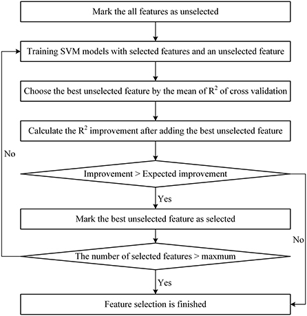
Figure 1. Flowchart of the StepSVM.

Prediction model construction

We chose 10 ML algorithms for prediction, including linear regression (LR), ridge regression (RR), Lasso, elastic net (EN), Huber regression (HR), K-nearest neighbor (KNN), support vector machine (SVM), random forest (RF), extreme gradient boosting (XGBoost), and artificial neural network (ANN).

We used 4 optimized feature sets and 10 ML algorithms to construct 40 regression models. All models were implemented in Python 3.8 using the scikit-learn (Pedregosa et al., 2011) and XGBoost (Chen and Guestrin, 2016) packages. The parameters of the models were determined by a cross-validated grid search.

Linear regression (LR)

LR is a simple multiple regression linear regression model. Usually, the LR coefficient is estimated using the ordinary least squares method, and the objective function of LR is:

J(θ)=12∑im(y(i) − θTx(i))2    (1) Ridge regression (RR)

RR is a modified ordinary least squares equal estimate. It gives up the unbiasedness of the least squares and makes the regression process more realistic at the cost of partial accuracy. It can prevent the model from overfitting by adding the L2-norm. The RR objective function is:

J(θ)=12∑im(y(i) − θTx(i))2+λ∑jnθj2    (2) Lasso

Lasso is a linear model that estimates sparse coefficients. Similar to RR, it consists of a linear model and an additional regularization term, but Lasso regression improves the ordinary least squares by adding the L1-norm. The Lasso regression objective function is:

J(θ)=12∑im(y(i) − θTx(i))2+λ∑jn|θj|    (3) Elastic net (EN)

EN is a linear regression model applying L1 and L2 regularization. It can not only remove invalid features as Lasso does but also has the stability of RR. The EN objective function is:

J(θ)=12∑im(y(i) − θTx(i))2+λ(ρ∑jn|θj|+(1−ρ)λ∑jnθj2)    (4) Huber regression (HR)

HR is a kind of robust estimation theory. It reduces the weight of outliers to reduce the impact of outliers on regression results. Its loss combines the advantages of the mean square error (MSE) and the mean absolute error (MAE).

J(θ)=∑i=1n(θ+Hδ(Sθ)θ)    (5)

Hδ(S)=,,,]},,,]},,,]},,,,,]}],"socialLinks":[,"type":"Link","color":"Grey","icon":"Facebook","size":"Medium","hiddenText":true},,"type":"Link","color":"Grey","icon":"Twitter","size":"Medium","hiddenText":true},,"type":"Link","color":"Grey","icon":"LinkedIn","size":"Medium","hiddenText":true},,"type":"Link","color":"Grey","icon":"Instagram","size":"Medium","hiddenText":true}],"copyright":"Frontiers Media S.A. All rights reserved","termsAndConditionsUrl":"https://www.frontiersin.org/legal/terms-and-conditions","privacyPolicyUrl":"https://www.frontiersin.org/legal/privacy-policy"}'>