Microorganisms play an important and far-reaching role in human life and greatly impact our health (Liang et al., 2018). Recent reports indicate that the human body is host to trillions of microorganisms (Hoffmann et al., 2016) and that the number of microorganisms in the human body far exceeds the number of human cells (Bocci, 1992). These microorganisms constitute the microbiota in the human body (Zhu et al., 2010). The microbiome plays a critical role in human physiology (Heintz-Buschart and Wilmes, 2018), helping the body’s intestinal tract to reduce the growth of pathogenic bacteria and infections and synthesizing some of the vitamins and amino acids needed by the body (Islam et al., 2022). Suppose the microbial community in the human body is out of balance. In that case, it can impair the function of the immune system, increase the risk of infection with pathogens (Pickard et al., 2017), lead to malnutrition or nutritional deficiencies (Burr et al., 2020), and contribute to the development of mental health-related problems such as anxiety and depression (Anisman et al., 2018), as well as metabolic diseases such as obesity and diabetes (Sanz et al., 2015). Of course, the microbiota can help the body regulate and prevent attacks from bacteria outside the body (Barr, 2017); for example, actinomycetes are a class of antibiotic-producing bacteria that produce a wide range of antibiotics such as streptomycin and tetracycline (Grasso et al., 2016). These antibiotics inhibit the growth of other pathogenic microorganisms and help protect the body from infection (Jagannathan et al., 2021). Therefore, predicting potential associations between microorganisms and diseases is vital for unraveling the complex mechanisms of disease occurrence and discovering potential biomarkers (Montaner et al., 2020). By inferring the interactions between microorganisms and diseases, we can better understand the diagnosis and prognosis of diseases and provide new ideas and methods for preventing, diagnosing, and treating diseases (Malla et al., 2019). As technology advances, we no longer rely solely on traditional biological methods to explore the association between microbes and disease (Gilbert et al., 2016). Instead, we are increasingly introducing computational modelling into our research to predict the role of microbes in disease occurrence, development, and treatment through techniques such as big data analytics and deep learning (Marcos-Zambrano et al., 2021), which are more practical and accurate (Najafabadi et al., 2015). Researchers have recently established a series of microbe-disease association databases to conduct an in-depth study of the potential link between microbes and diseases (Jin et al., 2022). These databases combine a large amount of microbial composition data and disease information. For example, the HMDAD database created by Ma et al. became the first to document human microbe-disease associations by manually organizing a large amount of public literature (Ma et al., 2017). This database covers 483 pieces of information about the association between 39 diseases and 292 microorganisms. Second, Janssens et al. created a microbial-disease association database called Disbiome by collecting 10,922 experimental records from 1,191 documents containing 372 diseases and 1,622 microorganisms (Janssens et al., 2018).

Researchers can explore and discover the relationships between microorganisms and different diseases using the above microbe-disease association database as the primary data. Moreover, these recent technological tools can be broadly categorized into four types, namely, network-based methods (Wu et al., 2018), matrix decomposition-based methods (Shen et al., 2021), traditional machine learning-based methods (Afshari et al., 2022), and graph neural network-based methods (Li et al., 2023).

In DuGEL, we use both Graph Convolutional Neural Network (GCN) and Graph Attention Network (GAT), where GCN is specifically designed to process graph data (Jin et al., 2021). GCN can learn feature representations at both node and graph levels, and it achieves the task of learning and predicting the representations of graph data by efficiently exploiting the connectivity relationships between the nodes (Zhou et al., 2023). By adaptively learning the attention weights between each node and its neighbouring nodes, GAT can better capture local structural information in graph data. The GAT introduction enriches the representational capabilities of the graph neural network, allowing it to perform well when dealing with complex graph-structured data (Munikoti et al., 2023). DuGEL can adapt to an extensive range of datasets with solid robustness.

Unlike the above methods, in this paper, we designed a new computational model called DuGEL based on the graph convolutional neural network and the graph attention network to infer possible microbe-disease associations. In DuGEL, we first downloaded known microbe-disease associations to form a heterogeneous microbe-disease network. Then, we input this network into a graph convolutional neural network and a graph attention network separately to obtain the local and global features of nodes in the network. Next, we spliced the outputs of the graph convolutional neural network and the graph attention network and then introduced a Long Short-Term Memory (LSTM) network to process the fused features. Finally, the output of the LSTM would be passed to a fully connected layer to infer potential associations between microbes and diseases. Experiments showed that DuGEL obtained satisfactory predictive performance with a 5-fold cross-validated auc of 0.9698 and 0.9119 for HMDAD and Disbiome datasets, respectively, and may be a potential tool for future microbe-disease association prediction.

HMDAD, constructed by Ma et al. (2017), and Disbiome (Janssens et al., 2018), constructed by Janssens et al., are the main publicly available biomedical databases containing microbe-disease association data. As shown in Table 1, HMDAD database covers 483 known microbe-disease associations, and processing these data, we ended up with 450 known microbial-disease associations. The HMDAD database provides a valuable information resource for studying microbial-disease relationships. In addition, the Disbiome, constructed by Janssens et al., is a publicly available database of microbe-disease associations. As shown in Table 1, Disbiome database collects 5,573 known associations from published academic papers for 240 diseases and 1,098 microorganisms. After de-duplication, we had 4,351 known microbe-disease associations covering 218 diseases and 1,052 microorganisms. Due to its extensive data collection and detailed information records, the Disbiome database has become a vital data support for research in this field.

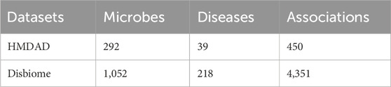
Table 1. The statistics of the two databases.

After acquiring the initial data, we performed data preprocessing steps to ensure the quality of the data and the validity of the model training. First, we removed all duplicate records to ensure that the association of each microbe with a disease was unique. Further, we converted the data into a uniform format to facilitate subsequent processing and model training. For simplicity, for each dataset, let M=m1m2,…,mNM denote the set of newly downloaded different microorganisms, and D=d1d2,…,dNd represent the set of newly downloaded different diseases. Thus, we can construct a primitive known microbe-disease association network Net=〈M∪ D,E as follows: for any given mi1≤i≤Nm and dj1≤j≤Nd, if and only if there is a known association between them, we assume that there is an edge belonging to E. Obviously, based on above definition, we can obtain an adjacency matrix A∈RNm×Nd as follows: for any given mi1≤i≤Nm and dj1≤j≤Nd if and only if there is an edge between them in E, there is Ai,j=1, otherwise, there is Ai,j=0.

As illustrated in above Figure 1, the DuGEL consists of the following five steps:

• Step 1: Construct a heterogeneous microbe-disease network based on newly downloaded known microbe-disease associations and multiple microbe and disease similarity metrics.

• Step 2: Feeding the heterogeneous microbe-disease network forward into a dual channel structure consisting of a Graph Convolutional Neural Network (GCN) and a Graph Attention Network (GAT), where the GCN is utilized to extract spatial features of nodes in the heterogeneous microbe-disease network from local to global, and the GAT is adopted to assign different importance to the neighbors of each node in the heterogeneous microbe-disease network as it is processed.

• Step 3: Splicing the outputs of GCN and GAT by simply fusing the information captured by GCN and GAT and combining structural and node characteristics and the importance between neighboring nodes.

• Step 4: Implementing a Long Short-Term Memory (LSTM) network to process the fused features, then feeding the output of LSTM into a fully connected layer to convert the high-level features captured by LSTM into the target output space.

• Step 5: By feeding the newly obtained feature vectors of the target output space into a Sigmoid function for binary prediction, potential associations between microbes and diseases can be finally computed.

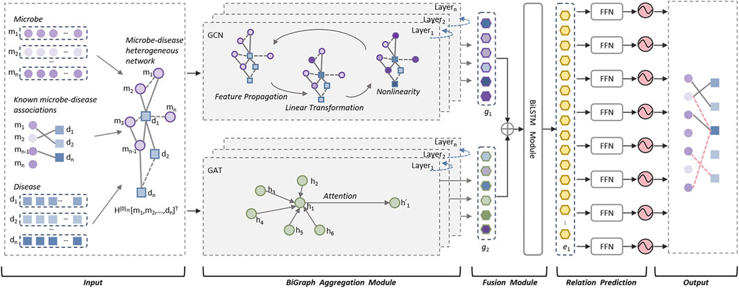
Figure 1. The structure of DuGEL.

In DuGEL, the input layer is the Microbe-Disease Association Representation Layer, is a component used to convert raw data of known microbe-disease associations into a structured data fame that can be processed by subsequent graph neural networks. Firstly, the newly collected microbe-disease association data need to be pre-processed to ensure consistency and accuracy. The preprocessed data will be used in turn to construct a binary microbe-disease association matrix M, which implies potential relationships between microorganisms and disease (Marsh and Zaura, 2017), and can be defined as follows: Given a microorganism m and a disease n, he known relationship between the microorganism and the disease can be characterized by a binary association matrix M∈Rm×n, where the matrix element Mij is 1 if there is a known association between the microorganism i and the disease j, and 0 otherwise. Each row of the matrix represents a microorganism, and each column represents a disease. The entries in the matrix indicate the presence or absence of an association. The graph structure G is obtained by the association matrix M, where the nodes in the graph are either microbe nodes or disease nodes, and if there is an association between a microbe node and a disease node (Abuin-Denis et al., 2024), i.e., Mij=1, then an edge exists between the nodes.

To enhance the prediction ability of DuGEL, similarity information is also fused in the representation layer (Feng et al., 2023), which contains the microbial similarity matrix Sm and the disease similarity matrix Sd. Among them, the microbial similarity matrix Sm captures similarities between different microorganisms based on genomic, phenotypic, or ecological characteristics. After the microbial similarity matrix Sm and disease similarity matrix Sd are constructed, we fuse this similarity information with the microbe-disease association matrix M to enhance the performance of the association prediction model. Therefore, at this point, we can obtain the association matrix that incorporates microbial similarity and disease similarity as a graph structure (Yu et al., 2024), which further serves as the initial input form for the dual graph-based feature extraction module. This graph structure captures direct associations and enables the model to learn a more comprehensive representation of features.

In addition, we will initialize each representative microbe or disease node in the graph with a feature vector. Formally, let Xm∈Rm×d represent the initial feature matrix for microbes and Xd∈Rn×d represent the initial feature matrix for diseases, where d is the dimension of the feature vector. The initial embeddings Xm and Xd are combined into a unified feature matrix X∈Rm+n×d. X is fed forward as input to the dual graph-based feature extraction module.

The microbe-disease association representation layer lays the foundation for the entire DuGEL model, and by meticulously structuring the input data, the layer ensures that subsequent graph neural networks are able to effectively capture both local and global patterns in the data. The construction of the graph enables the model to fully utilize all available information, thereby improving the accuracy and robustness of microbe-disease association predictions.

The Graph Convolutional Network (GCN) module extracts the spatial features of the graph by processing the microbe-disease feature matrix X to capture the intrinsic structural information of the graph. The spatial features represent the connections between nodes, including direct links (edges) and indirect influences through neighboring nodes. For example, in a microbe-disease graph, the direct association between a microbe and a disease, as well as second- or higher-order neighborhood relationships, contribute to the spatial information. The GCN extracts the features of the nodes by applying convolutional operations on the graph structure, and aggregates the information of the aggregated features of the local neighborhoods of each node by means of the layer-wise propagation rules (Du et al., 2024). The propagation rules of the GCN layers are defined as follows:

where Hl is the node representation X of the l nd layer, Wl whose initial input is, is the weight matrix of the l-th layer, σ denotes the nonlinear activation function, A^ is the representation of the adjacency matrix A plus the unitary matrix I, and D^ is the corresponding A^ degree matrix.

GCN effectively smoothies the feature representation over the graph structure and ensures that the representation of each node is influenced by its neighbors (Chen et al., 2021), thus capturing the local structure information. By aggregating a node’s neighbor information, the feature representation of a node is made to reflect its local graph structure. This aggregation operation is performed in each layer, and through the gradual aggregation of multiple layers (Liu et al., 2018), the GCN can capture a wider range of graph information. This is particularly important for microbe-disease association prediction, as some associations may not be directly visible, but indirectly inferred through multi-hop relationships.

The GAT sublayer enables the model to focus on the most relevant parts of the graph, thus capturing the importance of each neighboring node during the feature aggregation process. The advantage is that it can dynamically adjust the contribution of each neighbor to a node’s feature update, and by learning different attention weights, GAT can allocate different attention between different parts of the graph structure (Chatzianastasis et al., 2023). This is particularly useful when dealing with complex biological networks, where associations between microorganisms and diseases may have different biological significance and importance.

The dual graph feature extraction module can capture local and global information in the graph structure by combining GCN and GAT approaches. GCN emphasizes the aggregated features of a node’s local neighbors. At the same time, GAT dynamically adjusts the weights of the neighboring nodes through the attentional mechanism (Wang et al., 2022), thus providing more flexible and fine-grained control in the feature extraction process. This dual approach ensures that the model understands direct associations between microbes and diseases and identifies potential indirect relationships through graph structural features and attention weights. Combining these two approaches enables the DuGEL model to excel in microbe-disease association prediction tasks, providing more accurate and comprehensive predictions.

The dual graph feature extraction module plays a crucial role in the DuGEL model. Capturing complex graph structure information improves the model’s predictive ability and enhances its robustness and generalization ability.

In the dual graph feature extraction module, we extract two different feature representations through GCN and GAT. The task of the feature fusion layer is to effectively fuse these different features to obtain a comprehensive feature representation. The fusion operation can be realized in various ways, such as concatenation, weighted summing, or multilayer perceptron (MLP) (Afzal et al., 2023). Here, we adopt the concatenation operation to stitch together feature representations from different sub-networks to form a richer feature vector. Assuming that the feature representation extracted through GCN is HGCN and the feature representation extracted through GAT is HGAT, the fused feature representation Hfusion :

where ∥ represents the concatenation operation between the vectors; the fused feature matrix Hfusion ∈Rm+n×2d contains features extracted from two different viewpoints, providing a more comprehensive node representation.

After feature fusion, we need to further learn useful information from these high-dimensional features. The sequence learning layer is designed to capture the temporal or sequential dependencies between features to enhance the prediction capability (Yuan et al., 2023). By treating the node features as a sequence, the order in which node features are fed to the LSTM introduces a dependency chain. The model learns how the features of one node are influenced by or related to those of neighboring nodes. As illustrated in Figure 2, we introduce the Long Short-Term Memory Network (LSTM), which is capable of effectively remembering long-term dependencies and is suitable for processing sequence data (Yoo et al., 2023). The LSTM processes each node’s features across multiple time steps. Here, the “time steps” correspond to sequential relationships between node features derived from their embedding in the heterogeneous network. We represent the vector corresponding to the t-th time step in the matrix Hfusion ∈Rm+n×2d as Hfusiont∈R2d. The computational mechanism of the LSTM can be formally represented as follows:

where it, ft, and ot denote the activation vectors of the input, oblivion, and output gates, respectively, c∼t is the candidate cell state, ct and ht∈Rdl are the cell state and hidden state at time step, respectively, W and U are the learnable weight matrices, and b is the bias vector. dl is the dimensionality of the LSTM hidden layer. The output of the LSTM HLSTM =dltt=1m+n∈Rm+n×dl  combines information provided by the feature fusion layer, and captures through sequence learning the complex dependencies between features.

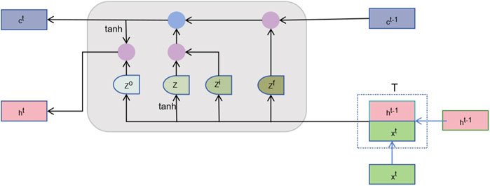
Figure 2. The structure of LSTM.

The feature fusion layer effectively integrates feature representations extracted from different perspectives, providing more comprehensive input data (Zhang et al., 2020). The sequence learning layer, on the other hand, further enhances the model’s predictive capability by capturing the temporal dependencies between features. Combining the two ensures the model can fully utilize all available information to achieve higher accuracy and robustness in microbe-disease association prediction tasks.

The feature representation HLSTM  output from the sequence learning layer is used as input to the fully connected layer for further processing. The fully connected layer maps the high-dimensional features to the final prediction results through a series of linear transformations and nonlinear activation functions (Feng et al., 2023). The computational process of the fully connected layer can be formally represented as:

where Wfc and b