An International Society of Magnetic Resonance in Medicine/National Institute of Standards and Technology (ISMRM/NIST) system phantom (High Precision Devices, Inc., Boulder, CO, USA) was used to evaluate the accuracy and repeatability of the QPM. The details of the ISMRM/NIST MRI system phantom configuration can be confirmed at the following site (https://qmri.com/qmri-solutions/t1-t2-pd-imaging-phantom/). The T1, T2, and PD values for each array are listed in Table 1.

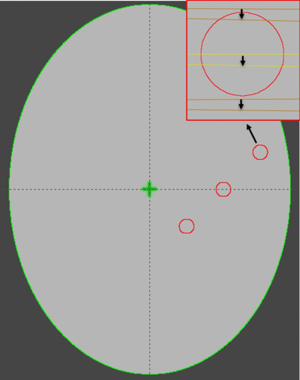
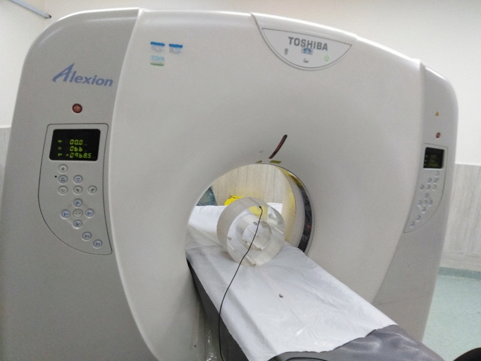
The ISMRM/NIST MRI system phantom was scanned using a 3 T MR scanner (Fujifilm, Ltd., Tokyo, Japan) equipped with a 15-channel head coil. The air-conditioning temperature of the MR scanner room was fixed at 22 °C, and a bandgap temperature sensor (standard accuracy 0.4 °C, resolution 0.01 °C) was placed 130 cm behind the gantry and 100 cm above the floor. The temperature measured hourly during the scans was 20.8 ± 0.5 °C. The ISMRM/NIST MRI system phantom was placed in the head coil such that the five plate surfaces were vertical to B0. The phantom was placed at the center of the gantry for 30 min before the scans. Axial images were scanned such that 14 spheres were visible in one image (Fig. 1). QPM, 2D inversion recovery spin echo (IR-SE), and 2D multi-echo RSGE were scanned from April 9, 2021, to April 24, 2021. The QPM, IR-SE, and RSGE were continuously scanned as a single set. Fifteen sets were obtained, with intervals larger than 6 h.

a sagittal T2WI of ISMRM/NIST MRI system phantom. The T1 array (solid line), T2 array (dashed line), and PD array (dotted line) are placed so that they are vertical to B0 (arrow). b Axial T2WI along with the T2 array

The optimization of QPM scan parameter sets (TR, TE, FA, and σ) were determined using the T1 and T2* values of the human brain tissues (gray matter (GM), white matter (WM), fat, and cerebrospinal fluid (CSF)) in Table 2 as target tissues [10]. Table 3 shows the scan parameter set of QPM used in this study. Other scan parameters were set as follows: FOV, 224 × 224mm2; slice thickness, 1.2 mm; number of slice, 187; acceleration factor, 1.2 × 1.2; matrix, 188 × 188; voxel size, 1.19 × 1.19 × 1.20; bandwidth, 90 kHz; number of signals averaged, 1. In this study, 11 different 3D images were acquired using these multiple imaging parameters in five scans, and the total acquisition time was 41 min and 26 s.

IR-SE for T1 value measurement and RSGE for T2* value measurement were performed using the imaging parameters in Table 4.

T1, T2*, and PD maps of QPM were created by performing the fitting process of Eq. (1) for each voxel using the acquired 11 3D images. Because the fitting process is limited to the calculation range of the T1 and T2* values (T1 value: 50–5600 ms, T2 value: 10–2800 ms), spheres No. 12–14 of T1 and T2 were excluded from the evaluation for accurate analysis. T1 and T2* values were calculated by IR-SE and RSGE, respectively, with the following procedure using MATLAB 2014b (MathWorks, Natick, MA, USA). The signal intensities M measured by each TI or TE image were substituted into Eqs. (2) and (3), respectively, and the T1 and T2* values were calculated by performing the nonlinear approximation process of the Levenberg–Marquardt method.

$$M = M0 (1-2 \left(\text\left(- T\text/T1\right)\right),$$

(2)

$$M = M0\text\left(-/^}\right),$$

(3)

where M0 is the equilibrium magnetization and M is any remnant magnetization that still presents at time t from any previous manipulations. Because T2* value analysis using targets with short T2 values might result in errors in T2* estimates due to noise effects caused by the inclusion of long TE signals, T2*map estimation was performed on two echoes at 4.6 ms and 14.6 ms for spheres with short T2 values (T2–11,10) and all seven echoes for other spheres to minimize the effect of noise.

We calculated the coefficients of variation (CV) from computer simulations that considered only normal distribution noise and compared it with the CV from T1 and T2* values obtained by QPM measurements to assess whether there are influences other than noise in the QPM measurements. Possible influences other than noise in the actual measurements include B1 intensity, spoilage accuracy, and liquid motion. The CV of QPM, IR-SE, and RSGE were calculated using computer simulations. The calculation algorithm used a Monte Carlo simulation to consider the noise effects. In this simulation, T2* is denoted as T2 because the effect of B0 inhomogeneities owing to differences in magnetic susceptibility is not included. All simulations were performed using Mathematica software (Wolfram Research, Champaign, IL, USA).

The CV of the 11 spheres in each of the T1 and T2 arrays were calculated using the following steps. Step 1: Substitute the T1 and T2 values and the 11 scan parameter sets of QPM into the QPM intensity function f(T1, T2, PD, B1, FA, TR, θ, TE). Here, the PD and B1 were set to 1. In this context, PD is set to 1 as the proportional coefficient to intensity values, and B1 is set to a uniform value of 1 as the spatial distribution coefficient of FA. This yielded 11 spheres × 11 parameter intensities for each of the T1 and T2 arrays. Step 2: Add 900 Gaussian noise to each of these 11 × 11 intensities and calculate 11 × 11 × 900 intensities with noise added. Step 3: Estimate T1 and T2 values for these intensities using QPM and obtain 11 spheres × 2 arrays × 900 pairs of (T1, T2). Step 4: Calculate CV from the estimated T1 and T2 values for each sphere.

The T1 and T2 values of the 11 spheres in the T1 array and the seven scan parameter sets of the IR-SE sequence with different TI were substituted into the T1 relaxation equation shown below to obtain 11 spheres × 7 parameter intensities.

$$I1=a1 }\left(-\text/T2\right) \left|1-2 B1 }\left(-\text/T1\right)\right|,$$

(4)

where \(I1\) is the intensity, \(a1\) is the proportionality coefficient, and \(\text\) is the inversion time. Nine-hundred Gaussian noises were added to these intensities to obtain 11 × 7 × 900 intensities with added noise. For each intensity, a least-squares fit of Eq. 2 was found to obtain the T1 value, and the CV was calculated from the 900 T1 values for each of the 11 spheres.

The T1 and T2 values of the 11 spheres in the T2 array and the seven scan parameter sets of the RSGE sequence with different TE were substituted into the T2 relaxation equation shown below to obtain 11 spheres × 7 parameter intensities.

$$I2=a2 }\left(-\text/T2\right),$$

(5)

where \(I2\) and \(a2\) are intensity and the proportionality coefficient, respectively. Nine hundred Gaussian noises were added to these intensities to obtain 11 × 7 × 900 intensities with added noise. For each intensity, a least-squares fit of Eq. 3 was used to obtain a T2 value, and the CV was calculated from the 900 T2 values for each of the 11 spheres. Because the signal intensity in the T2-10 and T2-11 spheres with short T2 values decayed in a short time, the T2 values were calculated from least-squares fitting using only the two scan parameters with short TE, as in the actual scans.

In this study, T1 maps of the QPM and IR-SE were used for T1 value evaluation, and T2* maps of the QPM and RSGE were used for T2* value evaluation. The PD maps obtained from QPM were used to evaluate the PD values. In addition to directly evaluating PD values, normalized PD with PD-14 (water, 100%), which means the percentage unit (pu) [12], was also evaluated because PD measured by QPM is a relative value. The measured value obtained from the PD map was defined as the unnormalized PD, and the normalized value from PD-14 was defined as the normalized PD. Region of interest (ROI) measurements for T1, T2*, and PD maps of the QPM were performed using ImageJ (National Institutes of Health, software version:1.52d). Rectangular ROIs (100 mm2) were placed at the center of the spheres by one of the authors (Y. H.). IR-SE and RSGE were measured by manually placing the ROIs in the same manner.

The mean and SD of T1 values were calculated and compared among the T1 maps of QPM, IR-SE, and the T1 reference values of the ISMRM/NIST MRI system phantom, and T2* values were calculated and compared among QPM, RSGE, and T2 reference values using intraclass correlation coefficients (ICC) and Bland–Altman plots. Additionally, ICC and Bland–Altman plots were generated using the normalized PD values obtained from QPM and the PD reference values of the ISMRM/NIST system phantom. JMP pro14 (SAS Institute Inc, Cary, NC, USA) and IBM SPSS Statistics version 21 (IMB, Armonk, NY, USA) were used for the statistical analyses. The repeatability of QPM was characterized by the CV and compared with the coefficient of variation of IR-SE and RSGE. CV was defined as the ratio between the standard deviation and mean T1, T2*, and PD values of 15 measurements. In addition, the measured CVs and computer simulations were compared to evaluate factors other than normally distributed noise that affect the quantitative values of QPM.