Clinical or biomedical data advances medical research by providing insights into patient health, disease progression, and treatment efficacy. It underpins new diagnostics, therapies, and personalized medicine, improving outcomes and understanding complex conditions. In predictive modeling, biomedical data is categorized as spatial, temporal, and spatio-temporal (Khalique et al., 2020; Veneri et al., 2012). Temporal data is key, capturing health evolution over time and offering insights into disease progression and treatment effectiveness. Time series data, collected at successive time points, shows complex patterns with short- and long-term dependencies, crucial for forecasting and analysis (Zou et al., 2019; Lai et al., 2018). Properly harnessed, this data advances personalized medicine and treatment optimization, making it essential in contemporary research.

Predictive modeling with artificial intelligence (AI) has gained significant traction across various domains, including manufacturing (Altarazi et al., 2019), heat transfer (Al-Hindawi et al., 2023; 2024), energy systems (Huang et al., 2024), and notably, the biomedical field (Cai et al., 2023; Patharkar et al., 2024). Predictive modeling in biomedical time series data involves various approaches for specific predictions and data characteristics. Forecasting models predict future outcomes based on historical data, such as forecasting blood glucose levels for diabetic patients using past measurements, insulin doses, and dietary information (Plis et al., 2014). Classification models predict categorical outcomes, like detecting cardiac arrhythmias from ECG data by classifying segments into categories such as normal, atrial fibrillation, or other arrhythmias, aiding in early diagnosis and treatment (Daydulo et al., 2023; Zhou et al., 2019; Chuah and Fu, 2007). Anomaly detection in biomedical time series identifies outliers or abnormal patterns, signifying unusual events or conditions. For example, monitoring ICU patients’ vital signs can detect early signs of sepsis (Mollura et al., 2021; Shashikumar et al., 2017; Mitra and Ashraf, 2018), enabling timely intervention.

Table 1 summarizes the example applications of these models within the context of biomedical time series.

Table 1. Overview of predictive modeling techniques for biomedical time series and their example applications across healthcare scenarios.

Regardless of the particular medical application or predictive model type used, models that manage biomedical time series data must tackle the intrinsic challenges posed by clinical and biomedical data. This includes various categories, such as electronic health records (EHRs), administrative data, claims data, patient/disease registries, health surveys, and clinical trials data. As illustrated in Table 2, each biomedical data category presents distinct challenges regarding quality, privacy, and completeness. During predictive modeling, further challenges arise. Specifically, we will investigate problems associated with missing data and imputation methods, the intricate nature of high-dimensional temporal relationships, and factors concerning the size of the dataset. Addressing these issues is crucial for developing strong and accurate predictive models in medical research.

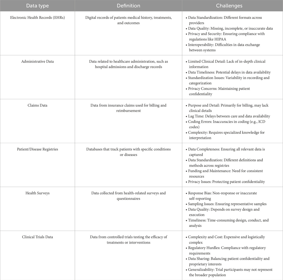
Table 2. Overview of clinical data types and challenges. This table lists the main types of clinical and biomedical data, their definitions, and key challenges.

Clinical data is often confronted with the issue of missing values, which can be caused by irregular data collection schedules or unexpected events (Xu et al., 2020). Medical measurements, recorded variably and at different times, may be absent, not documented, or affected by recording errors (Mulyadi et al., 2022), which makes the data irregular. Dealing with missing values in data sets usually involves either directly modeling data sets with missing values or filling in the missing values (a.k.a. imputation) to complete datasets for traditional analysis methods using data imputation techniques.

Current imputation techniques can be divided into four categories: case deletion, basic statistical imputation, machine learning-based imputation (Luo et al., 2018), and aggregating irregularly sampled data into discrete time periods (Ghaderi et al., 2023). Each of these methods comes with specific challenges in the context of handling biomedical temporal data. The deletion or omission of cases may lead to the loss of important information, particularly when the rate of missingness is high, which is critical in sensitive applications such as biomedical predictive modeling, where data is scarce and human lives are at risk. However, in certain cases, it is possible to do data omission without any potential risk to the outcome of the study. For instance, (Pinto et al., 2022), employs interrupted time series analysis to assess the impact of the “Syphilis No!” initiative in reducing congenital syphilis rates in Brazil. The results indicate significant declines in priority municipalities after the intervention. The study showcases the efficacy of public health interventions in modifying disease trends using statistical analysis of temporal data. Data collection needed to be conducted consistently over time and at evenly spaced intervals for proper analysis. To prevent bias due to the COVID-19 pandemic, December 2019 was set as the final data collection point, encompassing 20 months before the intervention (September 2016 to April 2018) and 20 months after the intervention (May 2018 to December 2019). This approach illustrates how the author addressed potential issues of irregular data or missing values in this context.

Contrary to data omission, statistical imputation techniques, such as mean or median imputation offer an alternative that reduces the effect of missing data, however, such methods do not take into account the temporal information but rather offer a summarized statistical imputation that often does not provide accurate replacement of the missing data. This could be critical in biomedical applications with scarce datasets, where the weight of a single data point could heavily affect the predictive power of the model. The use of machine learning-based imputation methods, such as Maximum Likelihood Expectation-Maximization, k-Nearest Neighbors, and Matrix Factorization, might offer a more accurate imputation that takes into account the specificity of the data point contrary to statistical aggregation methods, however, many of them still do not consider temporal relations between observations (Luo et al., 2018; Jun et al., 2019), and they usually are computationally expensive. Furthermore, without incorporating domain knowledge, these approaches can introduce bias and lead to invalid conclusions. Both machine learning and statistical techniques may not consider data distribution or variable relationships and may fail to capture complex patterns in multivariate time-series data due to the neglect of correlated variables, potentially resulting in underestimated or overestimated imputed values (Jun et al., 2019). Additionally, in real-time clinical decision support systems, timely and accurate data is crucial, as delays or errors in imputation can lead to incorrect decisions that directly affect patient outcomes. These systems demand high-speed processing, requiring imputation algorithms to be both computationally efficient and accurate. Moreover, the dynamic nature of clinical environments, where patient conditions can change rapidly, necessitates imputation methods that can adapt quickly to evolving data.

Aggregating measurements into discrete time periods can address irregular intervals, but it may lead to a loss of granular information (Ghaderi et al., 2023). Additionally, in time series prediction, missing values and their patterns are often correlated with target labels, referred to as informative missingness (Che et al., 2018). These limitations make it ill-advised to ignore, impute, or aggregate these values when handling biomedical time series data, but rather employ a model that is capable of handling the sparsity and the irregularity of clinical time series data.

Besides missing data challenges, hospitalized patients have a wide range of clinical events that are recorded in their electronic health records (EHRs). EHRs contain two different kinds of data: structured information, like diagnoses, treatments, medication prescriptions, vital signs, and laboratory tests, and unstructured data, like clinical notes and physiological signals (Xie et al., 2022; Lee and Hauskrecht, 2021), making them multivariate or high-dimensional (Niu et al., 2022).

The complexity of the relationships existing in such high-dimensional multivariate time series data can be difficult to capture and analyze. Analysts often try to predict future outcomes based on past data, and the accuracy of these predictions depends on how well the interdependencies between the various series are modeled (Shih et al., 2019). It is often beneficial to consider all relevant variables together rather than focusing on individual variables to build a prediction model, as this provides a comprehensive understanding of correlations in multivariate time series (MTS) data (Du et al., 2020). It thus becomes a requirement for predictive models employed in biomedical applications to take into account correlations among multiple dimensions and make predictions accordingly. It is equally crucial to ensure that only the features with a direct impact on the outcome are considered in the analysis. For instance, the study by Barreto et al. (2023) investigates the deployment of machine learning and deep learning models to forecast patient outcomes and allocate beds efficiently during the COVID-19 crisis in Rio Grande do Norte, Brazil. Out of 20 available features, nine were chosen based on their clinical importance and their correlation with patient outcomes, selected through discussions with clinical experts to guarantee the model’s accuracy and interpretability.

In addition to the inherent high dimensionality of biomedical data sourced from diverse platforms such as EHRs, wearable devices monitoring neurophysiological functions, and intensive care units tracking disease progression through physiological measurements (Allam et al., 2021), also display a natural temporal ordering. This temporal structure demands a specialized analytical approach distinct from that applied to non-temporal datasets (Zou et al., 2019). The temporal dependency adds significant complexity to modeling due to the presence of two distinct recurring patterns: short-term and long-term. For instance, short-term patterns may repeat daily, whereas long-term patterns might span quarterly or yearly intervals within the time series (Lai et al., 2018). Biomedical data often exhibit long-term dependencies, such as those seen in biosignals like electroencephalograms (EEGs) and electrocardiograms (ECGs), which may span tens of thousands of time steps or involve specific medical conditions such as acute kidney injury (AKI) leading to subsequent dialysis (Sun et al., 2021; Lee and Hauskrecht, 2021). Concurrently, short-term dependencies can manifest in immediate physiological responses to medical interventions, such as the administration of norepinephrine and subsequent changes in blood pressure (Lee and Hauskrecht, 2021). Another instance is presented by Valentim et al. (2022), who have created a model to forecast congenital syphilis (CS) cases in Brazil based on maternal syphilis (MS) incidences. The model takes into account the probability of proper diagnosis and treatment during prenatal care. It integrates short-term dependencies by assessing the immediate effects of prenatal care on birth outcomes, and long-term dependencies by analyzing syphilis case trends over a 10-year period. This strategy aids in enhancing public health decision-making and syphilis prevention planning.

Analyzing these recurrent patterns and longitudinal structures in biomedical data is essential to facilitate the creation of time-based patient trajectory representations of health events that facilitate more precise disease progression modeling and personalized treatment predictions (Allam et al., 2021; Xie et al., 2022). By incorporating both short-term fluctuations and long-term trends, robust predictive models can uncover hidden patterns in patient health records, advancing our understanding and application of digital medicine. Failing to consider these recurrent patterns can undermine the accuracy of time series forecasting in biomedical contexts such as digital medicine, which involves continuous recording of health events over time.

Additionally, early detection of diseases is of paramount importance. This can be achieved by utilizing existing biomarkers along with advanced predictive modeling techniques, or by introducing new biomarkers or devices aimed at early disease detection. For instance, early diagnosis of osteoporosis is essential to mitigate the significant socioeconomic impacts of fractures and hospitalizations. The novel device, Osseus, as cited by Albuquerque et al. (2023), addresses this by offering a cost-effective, portable screening method that uses electromagnetic waves. Osseus measures signal attenuation through the patient's middle finger to predict changes in bone mineral density with the assistance of machine learning models. The advantages of using Osseus include enhanced accessibility to osteoporosis screening, reduced healthcare costs, and improved patient quality of life through timely intervention.

The quantity of data available in a given dataset must be carefully considered, as it significantly influences model selection and overall analytical approach. For instance, when patients are admitted for brief periods, the clinical sequences generated are often fewer than 50 data points (Liu, 2016). Similarly, the number of data points for specific tests, such as mean corpuscular hemoglobin concentration (MCHC) lab results, can be limited due to the high cost of these tests, often resulting in less than 50 data points (Liu and Hauskrecht, 2015). Such limited data points pose challenges for predictive modeling, as models must be robust enough to derive meaningful insights from small samples without overfitting.

Conversely, some datasets may have a moderate sample length, ranging from 55 to 100 data points, such as the Physionet sepsis dataset (Reyna et al., 2019; 2020; Goldberger et al., 2000). These moderate-sized datasets offer a balanced scenario where the data is sufficient to train more complex models, but still requires careful handling to avoid overfitting and ensure generalizability.

In other cases, datasets can be extensive, particularly when long-span time series data is collected via sensor devices. These devices continuously monitor physiological parameters, resulting in large datasets with thousands of time steps (Liu, 2016). For example, wearable devices tracking neurophysiological functions or intensive care unit monitors can generate vast amounts of data, providing a rich source of information for predictive modeling. However, handling such large datasets demands models that are computationally efficient and capable of capturing long-term dependencies and complex patterns within the data.

The amount of data available is a major factor in choosing the appropriate model. Sparse datasets require models that can effectively handle limited information, often necessitating advanced techniques for data augmentation and imputation to make the most out of available data. Moderate datasets allow for the application of more sophisticated models, including machine learning and deep learning techniques, provided they are carefully tuned to prevent overfitting. Large datasets, on the other hand, enable the use of highly complex models, such as deep neural networks, which can leverage the extensive data to uncover intricate patterns and relationships.

The rest of the paper is structured as follows: In Section 2, statistical models are introduced. Section 3 covers machine learning models, while Section 4 focuses on deep learning models. This is followed by Section 5, which is a discussion section that summarizes the findings, discusses ensemble as well as hierarchical models, and explores future directions for the application of AI in clinical datasets. Finally, Section 6 concludes the paper.

(Yule, 1927) proposed an autoregressive (AR) model, and (Wold, 1948) introduced the Moving Averaging (MA) model, which were later combined by Box and Jenkins into the ARMA model (Janacek, 2010) for modeling stationary time series. The ARIMA model, an extension of ARMA, incorporates differencing to make the time series stationary before forecasting, represented by ARIMA (p,d,q), where p is the number of autoregressive terms, d is the degree of differencing, and q is the number of moving average terms. ARIMA models have been applied in real-world scenarios, such as predicting COVID-19 cases. Ding et al. (2020) used an ARIMA (1,1,2) model to forecast COVID-19 in Italy. In another study, (Bayyurt and Bayyurt, 2020), utilized ARIMA models for predictions in Italy, Turkey, and Spain, achieving a Mean Absolute Percentage Error (MAPE) value below 10%. Similarly, (Tandon et al., 2022), employed an ARIMA (2,2,2) model to forecast COVID-19 cases in India, reporting a MAPE of 5%, along with corresponding mean absolute deviation (MAD) and multiple seasonal decomposition (MSD) values.

When applying ARIMA models to biomedical data, we select the appropriate model using criteria like Akaike Information Criterion (AIC) or Bayesian information criterion (BIC), estimate parameters using tools like R or Python's statsmodels, and validate the model through residual analysis. ARIMA models are effective for univariate time series with clear patterns, supported by extensive documentation and software, but they require stationarity and may be less effective for data with complex seasonality. Moreover, if a time series exhibits long-term memory, ARIMA models may produce unreliable forecasts (Al Zahrani et al., 2020), signifying that they are inadequate for capturing long-term dependencies. Additionally, ARIMA models necessitate a minimum of 50 data points in the time series to generate accurate forecasts (Montgomery et al., 2015). Therefore, ARIMA models should not be used for biomedical data that require the modeling of long-term relationships or have a small number of data points.

Several extensions such as Seasonal ARIMA (SARIMA) have been introduced for addressing seasonality. For instance, the research by Liu et al. (2023) examined 10 years of inpatient data on Acute Mountain Sickness (AMS), uncovering evident periodicity and seasonality, thereby establishing its suitability for SARIMA modeling. The SARIMA model exhibited high accuracy for short-term forecasts, assisting in comprehending AMS trends and optimizing the allocation of medical resources. An additional extension of ARIMA, proposed for long-term forecasts, is ARFIMA. In the study by Qi et al. (2020), the Seasonal Autoregressive Fractionally Integrated Moving Average (SARFIMA) model was utilized to forecast the incidence of hemorrhagic fever with renal syndrome (HFRS). The SARFIMA model showed a better fit and forecasting accuracy compared to the SARIMA model, indicating its superior capability for early warning and control of infectious diseases by capturing long-range dependencies. Additionally, it is apparent that ARIMA models cannot incorporate exogenous variables. Therefore, a variation incorporating exogenous variables, known as the ARIMAX model, has been proposed. The study by Mahmudimanesh et al. (2022) applied the ARIMAX model to forecast cardiac and respiratory mortality in Tehran by analyzing the effects of air pollution and environmental factors. The key variables encompass air pollutants (CO, NO2, SO2, PM10) and environmental data (temperature, humidity). The ARIMAX model is selected for its capacity to include exogenous variables and manage non-static time series data.

For multi-step ahead forecasting in temporal prediction models, two methods exist. The first, known as the plug-in or iterated multi-step (IMS) prediction that involves successively using the single step predictor, treating each prediction as if it were an observed value to obtain the expected future value. The second approach is to create a direct multi-step (DMS) prediction as a function of the observations, and to select the coefficients in this predictor by minimizing the sum of squares of the multi-step forecast errors. Haywood and Wilson (2009) developed a test to decide which of two approaches is more dependable based on a given lead-time. In addition to this test, there are other ways to decide which technique is most suitable for forecasting multiple steps ahead. One of these methods can be used to decide the best choice for multi-step ahead prediction either for ARIMA or other types of models depending on the amount of historical data and the lead-time.

The EWMA method, based on Roberts (2000), uses first-order exponential smoothing as a linear combination of the current observation and the previous smoothed observation. The smoothed observation yt̃ at time t is given by the equation yt̃=λyt+(1−λ)yt−1̃, where λ is the weight assigned to the latest observation. This recursive equation requires an initial value y0̃. Common choices for y0̃ include setting it equal to the first observation y1 or the average of available data, depending on the expected changes in the process. The smoothing parameter λ is typically chosen by minimizing metrics such as Mean Squared Error (MSE) or MAPE (Montgomery et al., 2015).

Several modifications of simple exponential smoothing exist to account for trends and seasonal variations, such as Holt's method (Holt, 2004) and Holt-Winter's method (Winters, 1960). These can be used in either additive or multiplicative forms. For modeling and forecasting biomedical temporal data, the choice of method depends on the data characteristics. Holt's method is more appropriate for data with trends. On the other hand, EWMA is suitable for stationary or relatively stable data, making it effective in scenarios without a clear trend, such as certain biomedical measurements. For instance, Rachmat and Suhartono (2020) performed a comparative analysis of the simple exponential smoothing model and Holt’s method for forecasting the number of goods required in a hospital’s inpatient service, assessing performance using error percentage and MAD. Their findings indicated that the EWMA model outperformed Holt’s method, as it produced lower forecast errors. This outcome is logical since the historical data of hospitalized patients lack any discernible trend.

EWMA models are also intended for univariate, regularly-spaced temporal data, as demonstrated in the example above (Rachmat and Suhartono, 2020), which uses a single variable (number of goods) over a period of time as input for model construction. This model is not suitable for biomedical data that involves multiple variables influencing the forecast unless its extention for multivariate data is employed. As highlighted by De Gooijer and Hyndman (2006), there has been surprisingly little progress in developing multivariate versions of exponential smoothing methods for forecasting. Poloni and Sbrana (2015) attributes this to the challenges in parameter estimation for high-dimensional systems. Conventional multivariate maximum likelihood methods are prone to numerical convergence issues and high complexity, which escalate with model dimensionality. They propose a novel strategy that simplifies the high-dimensional maximum likelihood problem into several manageable univariate problems, rendering the algorithm largely unaffected by dimensionality.

EWMA models cannot directly handle data that is not evenly spaced, and thus cannot be used to directly model biomedical data with a large number of missing values without imputation. These models are capable of multi-step ahead prediction either through DMS or IMS approach. To emphasize long-range dependencies, the parameter λ can be set to a low value, while a higher value will give more importance to recent past value (Rabyk and Schmid, 2016). The range of λ values typically used for reasonable forecasting is 0.1–0.4, depending on the amount of historical data available for modeling (Montgomery et al., 2015).

Several regression models are available, and in this discussion, we focus on two specific types: multiple linear regression (MLR) (Galton, 1886; Pearson, 1922; Pearson, 2023) and multiple polynomial regression (MPR) (Legendre, 1806; Gauss, 1823). These models are particularly relevant for biomedical data analysis as they accommodate the use of two or more variables to forecast values. In MLR, there is one continuous dependent variable and two or more independent variables, which may be either continuous or categorical. This model operates under the assumption of a linear relationship between the variables. On the other hand, MPR shares the same structure as MLR but differs in that it assumes a polynomial or non-linear relationship between the independent and dependent variables. This review provides examination of these two regression models.

The estimated value of output y at time t, denoted as yt with a MLR model for a certain set of predictors is given by the following Equation 1.

where, Xt=(1,x1t,x2t,…,xkt) is a vector of k explanatory variables at time t, β=(β0,β1,…,βk)T are regression coefficients, and ϵt is a random error term at time t, t=1,…,N (Fang and Lahdelma, 2016). It can be solved with least squares method (Pearson, 1901) to obtain the regression coefficients.

R2 value can be calculated to check the accuracy of model fitting. The value of R2 that is closer to 1 indicates better model performance. Metrics such as Root Mean Squared Error (RMSE), Mean Absolute Percentage Error (MAPE), and Theil’s inequality coefficient (TIC) are commonly utilized to assess the forecasting model’s performance. While RMSE is scale-sensitive, MAPE and TIC are scale-insensitive. Lower values for these three metrics signify a well-fitting forecasting model.

Zhang et al. (2021) developed an MLR model aimed at being computationally efficient and accurate for forecasting blood glucose levels in individuals with type 1 diabetes. These MLR models can predict specific future intervals (e.g., 30 or 60 min ahead). The dataset is divided into training, validation, and testing subsets; missing values are handled using interpolation and forward filling, and the data is normalized for uniformity. The MLR model showed strong performance, especially in 60-min forward predictions, and was noted for its computational efficiency in comparison to deep learning models. It excelled in short-term time series forecasts with significant data variability, making it optimal for real-time clinical applications.

The estimated value of yt with say a second-order MPR model for a certain set of predictors is given by the following Equation 2.

where, β1t, β2t are regression coefficients, x1t,x2t,…,xnt are predictor variables, and ϵ is a random error. The ordinary least squares method (Legendre, 1806; Gauss, 1823) is applicable for solving this, similar to how it is used with MLR models. Furthermore, the evaluation metrics utilized for MLR are also suitable for MPR models.

Wu et al. (2021) utilized US COVID-19 data from January 22 to July 20 (2020), categorizing it into nationwide and state-level data sets. Positive cases were identified as Temporal Features (TF), whereas negative cases, total tests, and daily positive case increases were identified as Characteristic Features (CF). Various other features were employed in different manners, such as the daily increment of hospitalized COVID-19 patients. An MPR model was created for forecasting single-day outcomes. The model consisted of pre-processing and forecasting phases. The pre-processing phase included quantifying temporal dependency through time-window lag adjustment, selecting CFs, and performing bias correction. The forecasting phase involved developing MPR models on pre-processed data sets, tuning parameters, and employing cross-validation techniques to forecast daily positive cases based on state classification.

The various applications of multiple regression models stated above, linear or polynomial, reveal their inability to directly capture temporal patterns. Although these models can accommodate multiple input variables, their design limits them to forecasting a singular outcome with one model. One of the extentions proposed to tackle this problem is multivariate MLR (MVMLR). Suganya et al. (2020) employs MVMLR to forecast four continuous COVID-19 target variables (confirmed cases and death counts after one and 2 weeks) using cumulative confirmed cases and death counts as independent variables. The methodology includes data preprocessing, feature selection, and model evaluation using metrics like Accuracy, R2 score, Mean Absolute Error (MAE), Mean Squared Error (MSE), and Root Mean Squared Error (RMSE).

It is clear from the design of the regression models that they are unable to process missing input data. Unless all the predictor variables are present or substituted, the value of the output variable cannot be determined. Therefore, it becomes essential to apply imputation techniques prior to employing the regression models for forecasting.

The regression models do not usually require a large amount of data; it has been demonstrated to be effective with as few as 15 data points per case (Filipow et al., 2023). Multi-step ahead prediction can be accomplished with either IMS or DMS approaches when dealing with temporal data like previous cases. Nonetheless, as mentioned previously, since these methods do not inherently capture temporal dependencies, forecasts can be generated as long as the temporal order is maintained while training, and testing the model.

The origin of Support Vector Machines (SVMs) can be traced back to Vapnik (1999). Initially, SVMs were designed to address the issue of classification, but they have since been extended to the realm of regression or forecasting problems (Vapnik et al., 1996). The SVR approach has the benefit of transforming a nonlinear problem into a linear one. This is done by mapping the data set x into a higher-dimensional, linear feature space. This allows linear regression to be performed on the new feature space. Various kernels are employed to convert non-linear data into linear data. The most commonly used are linear kernel, polynomial kernel, and radial basis or Gaussian kernel.

Upon transforming a nonlinear dataset x into a higher-dimensional, linear feature space, the prediction function f(x) is expressed by Equation 3.

The SVR algorithm solves a nonlinear regression problem by transforming the training data xi (where i ranges from one to N, with N being the size of the training data set) into a new feature space, denoted by ϕ(x). This transformation allows establishing a linear relationship between input and output, using the weight matrix w and bias matrix b to further refine the model.

In SVR, selecting optimal hyperparameters (C,ϵ) is crucial for accurate forecasting. The parameter C controls the balance between minimizing training error and generalization. A higher C reduces training errors but may overfit, while a lower C results in a smoother decision function, possibly sacrificing training accuracy. The parameter ϵ sets a tolerance margin where errors are not penalized, forming an ϵ-tube around predictions. A larger ϵ simplifies the model but may underfit, whereas a smaller ϵ provides more detail, potentially leading to overfitting. Optimal values for C and ϵ may require additional methods (Liu et al., 2021).

SVR is often combined with other algorithms for parameter optimization. Evolutionary algorithms frequently determine SVR parameters. For example, Hamdi et al. (2018) used a combination of SVR and differential evolution (DE) to predict blood glucose levels with continuous glucose monitoring (CGM) data. The DE algorithm was used to determine the optimal parameters of the SVR model, which was then built based on these parameters. The model was tested using real CGM data from 12 patients, and RMSE was used to evaluate its performance for different prediction horizons. The RMSE values obtained were 9.44, 10.78, 11.82, and 12.95 mg/dL for prediction horizons (PH) of 15, 30, 45, and 60 min, respectively. It should be noted that when these evolutionary algorithms are employed for determining parameters, SVR encounters notable disadvantages, including a propensity to get stuck in local minima (premature convergence).

Moreover, SVR can occasionally lack robustness, resulting in inconsistent outcomes. To mitigate these challenges, hybrid algorithms and innovative approaches are applied. For instance, Empirical Mode Decomposition (EMD) is employed to extract non-linear or non-stationary elements from the initial dataset. EMD facilitates the decomposition of data, thereby improving the effectiveness of the kernel function Fan et al. (2017).

Essentially, SVR is an effective method for dealing with MTS data (Zhang et al., 2019). SVR, which operates on regression-based extrapolation, fits a curve to the training data and then uses this curve to predict future samples. It allows for continuous predictions rather than only at fixed intervals, making it applicable to irregularly spaced time series (Godfrey and Gashler, 2017). Nonetheless, due to its structure, SVR struggles to capture complex temporal dependencies (Weerakody et al., 2021).

It is suitable for smaller data sets as the computational complexity of the problem increases with the size of the sample Liu et al. (2021). It excels at forecasting datasets with high dimensionality Gavrishchaka and Banerjee (2006) due to the advanced mapping capabilities of kernel functions Fan et al. (2017). Additionally, multi-step ahead prediction in the context of SVR’s application to temporal data can be achieved either with the DMS or IMS approach (Bao et al., 2014).

In 1951, Evelyn Fix and Joseph Hodges developed the KNN algorithm for discriminant examination analysis (Fix and Hodges, 1989). This algorithm was then extended to be used for regression or forecasting. The KNN method assumes that the current time series segment will evolve in the future in a similar way to a past time series segment (not necessarily a recent one) that has already been observed (Kantz and Schreiber, 2004). The task is thus to identify past segments of the time series that are similar to the present one according to a certain norm. Given a time series yN(N) with N samples, the segment made of the last m samples is denoted as yM(N), reflecting the current disturbance pattern. The KNN algorithm searches for k past time series intervals most comparable to yM(N) within the memory yN(N) using various distance metrics. For each nearest neighbor, a following time series of length h is generated, known as prediction contributions. Forecasting can then be done using unweighted or weighted approaches. In the unweighted approach, the prediction is the mean of the prediction contributions. In the weighted approach, the prediction is a weighted average based on the distance of each nearest neighbor from the current segment. Weights are assigned inversely proportional to the distances.

Gopakumar et al. (2016) employed the KNN algorithm to forecast the total number of discharges from an open ward in an Australian hospital, which lacked real-time clinical data. To estimate the next-day discharge, they used the median of similar discharges from the past. The quality of the forecast was evaluated using the mean forecast error (MFE), MAE, symmetric MAE (SMAPE), and RMSE. The results of these metrics were reported to be 1.09, 2.88, 34.92%, and 3.84, respectively, with an MAE error improvement of 16.3% over the naive forecast.

KNN regression is viable for multivariate temporal datasets, as illustrated by Al-Qahtani and Crone (2013). Nevertheless, its forecasting accuracy diminishes as the dimensionality of the data escalates. Consequently, it is critical to meticulously select pertinent features that impact the target variable to enhance model performance.

KNN proves effective for irregular temporal datasets (Godfrey and Gashler, 2017) due to its ability to identify previous matching patterns rather than solely depending on recent data. This distinctive characteristic renders KNN regression a favored choice for imputing missing data (Aljuaid and Sasi, 2016) prior to initiating any forecasting. Furthermore, it excels in capturing seasonal variations or local trends, such as aligning the administration of a medication that elevates blood pressure with a low blood pressure condition. Conversely, its efficacy in identifying global trends is limited, particularly in scenarios like septic shock, where multiple health parameters progressively deteriorate over time (Weerakody et al., 2021).

The KNN algorithm necessitates distance computations for k-nearest neighbors. Selecting an appropriate distance metric aligned with the dataset's attributes is essential, with Euclidean distance being prevalent, though other metrics may be more suitable for specific datasets. Ehsani and Drabløs (2020) examines the impact of various distance measures on cancer data classification, using both common and novel measures, including Sobolev and Fisher distances. The findings reveal that novel measures, especially Sobolev, perform comparably to established measures.

As the size of the training dataset increases, the computational demands of the algorithm also rise. To mitigate this issue, approximate nearest neighbor search algorithms can be employed (Jones et al., 2011). Furthermore, the algorithm requires a large amount of data to accurately detect similar patterns. Several methods have been suggested to accelerate the process; for example, (Garcia et al., 2010), presented two GPU-based implementations of the brute-force kNN search algorithm using CUDA and CUBLAS, achieving speed-ups of up to 64X and 189X over the ANN C++ library on synthetic data.

Similarly to other forecasting models, KNN is applicable for multistep ahead predictions using strategies such as IMS or DMS (Martínez et al., 2019). It is imperative to thoroughly analyze the clinical application and characteristics of the clinical data prior to employing KNN regression for forecasting, given its unique attributes. Optimizing the number of neighbors (k) and the segment length (m) through cross-validation is crucial. Employing appropriate evaluation metrics (e.g., MFE, MAE, SMAPE, RMSE) is necessary to assess the model’s performance.

Random Forests (RFs), introduced by Breiman (2001), are a widely-used forecasting data mining technique. According to Bou-Hamad and Jamali (2020), they are tree-based ensemble methods used for predicting either categorical (classification) or numerical (regression) responses. In the context of regression, known as Random Forest Regression (RFR), RF models strive to derive a prediction function f(x) that reduces the expected value of a loss function L(Y,f(X)), with the output Y typically evaluated using the squared error loss. RFR builds on base learners, where each learner is a tree trained on bootstrap samples of the data. The final prediction is the average of all tree predictions as shown by Equation 4.

where K is the number of trees, and lk(x) is the k-th tree. Trees are constructed using binary recursive partitioning based on criteria such as MSE.

Zhao et al. (2019) developed a RFR model to forecast the future estimated glomerular filtration rate (eGFR) values of patients to predict the progression of Chronic Kidney Disease (CKD). The data set used was from a regional health system and included 120,495 patients from 2009 to 2017. The data was divided into three tables: eGFR, demographic, and disease information. The model was optimized through grid-search and showed good fit and accuracy in forecasting eGFR for 2015–2017 using the historical data from the past years. The forecasting accuracy decreased over time, indicating the importance of previous eGFR records. The model was successful in predicting CKD stages, with an average R2 of 0.95, 88% Macro Recall, and 96% Macro Precision over 3 years.

The study presented in Zhao et al. (2019) indicates that RFR is effective for forecasting multivariate data. Another research by Hosseinzadeh et al. (2023) found that RFR performs better with multivariate data than with univariate data, especially when the features hold substantial information about the target. Research by Tyralis and Papacharalampous (2017) indicated that RF incorporating many predictor variables without selecting key features exhibited inferior performance relative to other methods. Conversely, optimized RF utilizing a more refined set of variables showed consistent reliability, highlighting the importance of thoughtful variable selection.

Similar to SVR, RFR is able to process non-linear information, although it does not have a specific design for capturing temporal patterns (Helmini et al., 2019). RFR is capable of handling irregular or missing data. El Mrabet et al. (2022) compared RFR for fault detection with Deep Neural Networks (DNNs), and found that RFR was more resilient to missing data than DNNs, showing its superior ability to manage missing values. To apply RFR to temporal data, it must be suitably modeled. As an example, Hosseinzadeh et al. (2023) has demonstrated one of the techniques, which involves forecasting stream flow by modeling the RFR as a supervised learning task with 24 months of input data and corresponding 24 months of output sequence. The construction of sequences involves going through the entire data set, shifting 1 month at a time. The study showed that extending the look-back window beyond a certain time frame decreases accuracy, indicating RFR’s difficulty in capturing long-term dependencies when used in temporal modeling context. For a forecasting window of 24 months, the look-back window must be at least 24 months to avoid an increase in MAPE. This implies that although RFR can be used for temporal modeling, its effectiveness is more in capturing short-term dependencies rather than long-term ones. The experiments conducted by Tyralis and Papacharalampous (2017) also support this, showing that utilizing a small number of recent variables as predictors during the fitting process significantly improves the RFR’s forecasting accuracy.

RFR can be used to forecast multiple steps ahead, similar to other regression models used for temporal forecasting (Alhnaity et al., 2021). Regarding data management, RFR necessitates a considerable volume of data to adjust its hyperparameters. It can swiftly handle such extensive datasets, leading to a more accurate model (Moon et al., 2018).