Million-scale training dataset

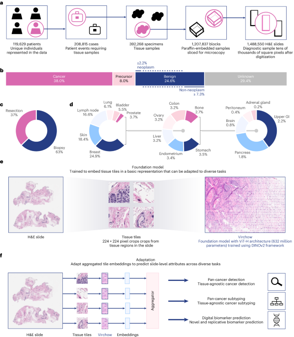
Institutional review board review was not applicable for the research described in this study. This research study was conducted retrospectively from deidentified data licensed to Paige.AI, Inc. from MSKCC. The data used in this study were all collected originally for clinical use by MSKCC in the practice setting and are therefore considered secondary data. Only data previously deidentified by MSKCC were utilized in the analysis, and unique patient identifiers were completely removed from the analytical dataset. To the best of our knowledge, MSKCC has not transferred any data for which the applicable patient has not consented to or otherwise agreed to MSKCC’s Notice of Privacy Practices or a substantially similar notice, waiver or consent. The training digital pathology dataset comprises 1,488,550 WSIs derived from 119,629 patients. These WSIs are all stained with H&E, a routine stain that stains the nuclei blue and the extracellular matrix and cytoplasm pink. The WSIs are scanned at ×20 resolution or 0.5 mpp using Leica scanners. Seventeen high-level tissue groups are included, as illustrated in Fig. 1c.

WSIs are gigapixels in size and are challenging to use directly during training. Instead, Virchow was trained on tissue tiles that were sampled from foreground tissue in each WSI. To detect foreground, each WSI was downsampled 16× with bilinear interpolation, and every pixel of the downsampled image was evaluated as to whether its hue, saturation and value were within [90, 180], [8, 255] and [103, 255], respectively. All non-overlapping 224 × 244 tiles containing at least 25% tissue by area were collected. Virchow was trained on 2 billion tiles sampled randomly with replacement from approximately 13 billion available tissue tiles.

Virchow architecture and training

Virchow employs the ViT ‘huge’ architecture (ViT-H/14), a ViT34 with 632 million parameters that was trained using the DINO v.2 (ref. 33) self-supervised learning algorithm, as illustrated in Extended Data Fig. 1. The ViT is an adaptation of the transformer model for image analysis, treating an image as a sequence of patches. These patches are embedded and processed through a transformer encoder that uses self-attention mechanisms. This approach allows ViT to capture complex spatial relationships across the image. DINO v.2 is based on a student–teacher paradigm: given a student network and a teacher network, each using the same architecture, the student is trained to match the representation of the teacher. The student network is information-limited, as it is trained using noisy variations of input tiles. The teacher network is a slowly updated exponential moving average of past student networks; matching the teacher achieves an effect similar to ensembling over prior student predictions57. The student learns a global representation of an image by matching the teacher’s class token, as well as local representations by matching the teacher’s patch tokens. Patch tokens are only matched for a select subset of tokens that are randomly masked out of an input image (for the student), as done in masked image modeling58. Additional regularization helps DINO v.2 trained models outperform the earlier DINO variant25.

The default hyperparameters for training the DINO v.2 model were used for Virchow as detailed in ref. 33 with the following changes: a teacher temperature schedule of 0.04–0.07 in 186,000 iterations and a reciprocal square root learning rate schedule with a warmup of 495,000 iterations (instead of 100,000) and linear cooldown to 0.0 for the last 819,200 iterations29. Virchow was trained using AdamW (β1 = 0.9, β2 = 0.999) with float16 precision. Note that with ViT-H, we used 131,072 prototypes (and thus 131,072-dimensional projection heads). During distributed training, each mini-batch was sampled by randomly selecting one WSI per graphics processing unit and 256 foreground tiles per WSI.

Pan-cancer detection

Specimen-level pan-cancer detection requires a model that aggregates foundation model embeddings from all foreground tiles of all WSIs in a specimen to detect the presence of cancer. All pan-cancer detection models trained in this work use an Agata10 aggregator model, weakly supervised with multiple-instance learning (see Extended Data Fig. 2 for architecture details).

Embedding generation

For a 224 × 224 input tile image, a Virchow embedding is defined as the concatenation of the class token and the mean across all 256 of the other predicted tokens. This produces an embedding size of 2,560 (1,280 × 2). For Phikon, only the class token is used, as recommended by ref. 37. For CTransPath, the mean of all tokens is used as there is no class token.

Training data

To train the aggregator model, we prepared a subset of the training dataset used for training Virchow (see ‘Million-scale training dataset’ in Methods for details), combined with specimen-level labels (block-level for prostate tissue) indicating the presence or absence of cancer extracted from synoptic and diagnostic reports. The training and validation datasets combined consist of 89,417 slides across 40,402 specimens. See Extended Data Fig. 4b for the training data distribution, stratified by WSI tissue type and cancer status.

Aggregator training

The Agata aggregator was trained as described in Extended Data Fig. 2. Because the label is at the level of the specimen, all tiles belonging to the same specimen need to be aggregated during training. Training using embeddings for all tiles of a specimen is prohibitively memory-intensive. We thus select the slide with the highest predicted cancer probability per specimen and backpropagate the gradients only for that slide.

As baselines, aggregators using Phikon and CTransPath embeddings were also trained. All aggregators were trained for 25 epochs using the cross-entropy loss and the AdamW59 optimizer with a base learning rate of 0.0003. During each training run, the checkpoint with the highest validation AUC was selected for evaluation.

Testing dataset

The pan-cancer detection models are evaluated on a combination of data sourced from MSKCC and external institutions. None of the patients in the evaluation set were seen during training. The dataset contains 22,932 slides from 6,142 specimens across 16 cancer types. We hypothesize that the more data the foundation model is trained on, the better the downstream task performance, especially on data-constrained tasks. To test this hypothesis, we categorize cancer types into common or rare cancer groups. According to the NCI, rare cancers are defined as those occurring in fewer than 15 people out of 100,000 each year in the United States46. Based on this definition, common cancer comprises 14,179 slides from 3,547 specimens originating in breast, prostate, lung, colon, skin, bladder, uterus, pancreas and H&N, and rare cancer comprises 8,753 slides from 2,595 specimens originating in liver, stomach, brain, ovary, cervix, testis and bone. Note that each cancer type is determined by its tissue of origin and thus may appear in any tissue (as primary or metastatic cancer). On the other hand, benign specimens for each cancer type were sampled only from the tissue of origin. For example, the liver stratum contains 182 liver specimens with liver cancer (primary), 18 non-liver specimens with liver cancer (metastatic) and 200 benign liver specimens. For each cancer type, Fig. 2a shows the distribution between primary and metastatic cancer, and Extended Data Fig. 4a additionally shows the number of benign specimens.

The testing dataset includes 15,622 slides from 3,033 specimens collected at MSKCC (denoted as ‘Internal’ in Fig. 2b), in addition to 7,310 slides (3109 specimens) sent to MSKCC from institutions around the world (‘External’ in Fig. 2b). See Extended Data Fig. 4a for the testing data distribution, stratified by cancer type (for specimens with cancer) or by tissue type (for benign specimens).

Label extraction

To establish the clinical cancer diagnosis at the specimen level, a rule-based natural language processing system was employed. This system decomposes case-level reports to the specimen level and analyzes the associated clinical reports with each specimen, thereby providing a comprehensive understanding of each case.

Statistical analysis

The performance of the three models is compared using two metrics: AUC and specificity at 95% sensitivity. AUC is a suitable general metric because it does not require selecting a threshold for the model’s probability outputs, something that may need tuning for different data subpopulations. Specificity at 95% sensitivity is informative because a clinical system must be not only sensitive but also specific in practice. For AUC, the pairwise DeLong’s test60 with Holm’s method61 for correction is applied to check for statistical significance. For specificity, first Cochran’s Q test62 is applied, and then McNemar’s test63 is applied post hoc for all pairs with Holm’s method for correction. The two-sided 95% confidence intervals in Fig. 2b–e and Extended Data Fig. 3 were calculated using DeLong’s method60 for AUC and Wilson’s method64 for specificity. In addition to overall analysis, stratified analysis is also conducted for each cancer type.

Clinical evaluation datasets

To perform an extensive evaluation of the Virchow-based pan-cancer detection model, we employ seven additional datasets (see Supplementary Table 2.1 for details). One of these datasets is pan-tissue, and the rest are single-tissue datasets containing tissues for which Paige has clinical products: that is, prostate, breast and lymph node.

Pan-tissue product benchmark

This dataset contains 2,419 slides across 18 tissue types (Supplementary Table 2.2). Each slide is individually inspected by a pathologist and labeled according to presence of invasive cancer. An important distinction between the testing dataset in ‘Pan-cancer detection’ and this dataset is that the former is stratified according to origin tissue in cancerous specimens, whereas the latter is stratified according to tissue type for all slides, as it is more relevant in a clinical setting. We use this dataset to identify failure modes of the pan-cancer detection model.

Prostate product benchmark

This dataset contains 2,947 blocks (3,327 slides) of prostate needle core biopsies (Supplementary Table 2.7). Labels for the blocks are extracted from synoptic reports collected at MSKCC. This dataset has been curated to evaluate the standalone performance of Paige Prostate Detect, which is a tissue-specific, clinical-grade model. We use this dataset to compare the pan-cancer detection model to Paige Prostate Detect.

Prostate rare variants benchmark

This dataset contains 28 slides containing rare variants of prostate cancer (neuroendocrine tumor, atrophic, small lymphocytic lymphoma, foamy cell carcinoma, follicular lymphoma) and 112 benign slides (Supplementary Table 2.8). Cancerous slides are curated and labeled by a pathologist, and are appended with slides from benign blocks determined from synoptic reports collected at MSKCC.

Breast product benchmark

This dataset contains 190 slides with invasive cancer and 1,501 benign slides, labeled individually by a pathologist according to presence of atypical ductal hyperplasia, atypical lobular hyperplasia, lobular carcinoma in situ, ductal carcinoma in situ, invasive ductal carcinoma, invasive lobular carcinoma and/or other subtypes (Supplementary Table 2.5). This dataset has been curated to evaluate the standalone performance of Paige Breast, which is a tissue-specific, clinical-grade model. We use the subtype information for stratified analysis.

Breast rare variants benchmark

This dataset contains 23 cases of invasive ductal carcinoma or invasive lobular carcinoma (as control), 75 cases of rare variants (adenoid cystic carcinoma, carcinoma with apocrine differentiation, cribriform carcinoma, invasive micropapillary carcinoma, metaplastic carcinoma (matrix producting subtype, spindle cell and squamous cell), mucinous carcinoma, secretory carcinoma and tubular carcinoma) and 392 benign cases (total 5,031 slides). Cancerous cases are curated by a pathologist, and are appended with benign cases determined from synoptic reports collected at MSKCC. See Supplementary Table 2.6 for details.

BLN

This dataset contains 458 lymph node slides with metastasized breast cancer and 295 benign lymph node slides (Supplementary Table 2.3). Each slide has been labeled by a pathologist according to presence of invasive cancer, and the largest tumor on the slide is measured to categorize the tumor into macrometastasis, micrometastasis or infiltrating tumor cells. We use the categories for stratified evaluation.

Lymph node rare variants benchmark

This dataset contains 48 specimens of rare variants of cancers (diffused large B-cell lymphoma, follicular lymphoma, marginal zone lymphoma, Hodgkin’s lymphoma) selected by a pathologist and 192 benign specimens determined from synoptic reports collected at MSKCC (Supplementary Table 2.4).

Biomarker detection

We formulated each biomarker prediction task as a binary pathology case classification problem, where a positive label indicates the presence of the biomarker. Each case consists of one or more H&E slides that share the same binary label. We randomly split each dataset into training and testing subsets, ensuring no patient overlap, as shown in Supplementary Table 3.1. The clinical importance of each biomarker is described below.

Colon-MSI

Microsatellite instability (MSI) occurs when DNA regions with short, repeated sequences (microsatellites) are disrupted by single nucleotide mutations, leading to variation in these sequences across cells. Normally, mismatch repair (MMR) genes (MSH1, MSH2, MSH6, PMS2) correct these mutations, maintaining consistency in microsatellites. However, inactivation of any MMR gene (through germline mutation, somatic mutation or epigenetic silencing) results in an increased rate of uncorrected mutations across the genome. MSI is detected using polymerase chain reaction or next-generation sequencing, which identifies a high number of unrepaired mutations in microsatellites, indicative of deficient mismatch repair (dMMR). Microsatellite instability high (MSI-H) suggests dMMR in cells, identifiable via IHC, which shows absent staining for MMR proteins. MSI-H is present in approximately 15% of colorectal cancers (CRCs), often linked to germline mutations that elevate hereditary cancer risk. Consequently, routine MSI or IHC-based dMMR screening is recommended for all primary colorectal carcinoma samples. The Colon-MSI dataset, comprising 2,698 CRC samples with 288 MSI-H/dMMR positive cases, uses both IHC and MSK-IMPACT sequencing for dMMR and MSI-H detection, prioritizing IHC results when both test outcomes are available.

Breast-CDH1

The biallelic loss of cadherin 1 (CDH1) gene (encoding E-cadherin) is strongly correlated with lobular breast cancer and a distinct histologic phenotype and biologic behavior65. CDH1 inactivating mutations associated with loss of heterozygosity or a second somatic loss-of-function mutation as determined by MSK-IMPACT sequencing test results were considered as ‘CDH1 biallelic mutations’. The CDH1 dataset comprises a total of 1,077 estrogen receptor-positive (ER+) primary breast cancer samples, in which 139 were positive and 918 were negative. The remaining 20 samples with other types of variants—that is, monoallelic mutations—were excluded.

Bladder-FGFR

The fibroblast growth factor receptor (FGFR) is encoded by four genes (FGFR1, FGFR2, FGFR3, FGFR4). FGFR gene alterations screening in bladder carcinoma allows the identification of patients targetable by FGFR inhibitors. Anecdotal experience from pathologists suggested there may be a morphological signal for FGFR alterations66. The FGFR binary label focuses on FGFR3 p.S249C, p.R248C, p.Y373C, p.G370C mutations, FGFR3-TACC3 fusions and FGFR2 p.N549H, pN549K, p.N549S, p.N549T mutations based on data from the MSK-IMPACT cohort. From the total of 1,038 samples (1,087 WSIs), 26.2% have FGFR3 alterations.

Lung-EGFR

The EGFR oncogenic mutation screening in non-small cell lung cancer is essential to determine eligibility for targeted therapies in late stage non-small cell lung cancer67. The oncogenic status of EGFR mutation was determined based on OncoKB annotation68. EGFR mutations with any oncogenic effect (including predicted/likely oncogenic) were defined as positive label, and EGFR mutation with unknown oncogenic status were excluded.

Prostate-AR

The AR amplification/overexpression was found in 30%–50% of castration resistant prostate cancers and was associated with resistance to androgen deprivation therapy. In the AR dataset, the copy number amplification of AR was determined by MSK-IMPACT sequencing test, for which the fold change was greater than two.

Gastric-HER2

Human epidermal growth factor receptor 2 (HER2) overexpression and/or amplification are much more heterogeneous in gastric cancer compared to breast cancer. Approximate 20% of gastric cancer patients are found to correlate with HER2 overexpression/high-level amplification, and they would be likely to benefit from treatment with an anti-HER2 antibody therapy. Here, a HER2 IHC result of 2+, confirmed positive with fluorescence in situ hybridization (FISH) or an IHC result of 3+ were considered HER2 amplification.

Endometrial-PTEN

PTEN is the most frequently mutated tumor suppressor gene in endometrial cancer. The presence of PTEN mutation showed to be significantly associated with poorer prognosis in survival and disease recurrence. The oncogenic status of PTEN mutation was determined based on MSK-IMPACT sequencing and OncoKB annotation68. The variants associated with any oncogenic effect (including predicted and/or likely oncogenic) were defined as positive label for PTEN mutations, and variants with unknown oncogenic status were excluded.

Thyroid-RET

RET mutations were highly associated with medullary thyroid cancer, which accounts for about 5–10% of all thyroid cancer. Screening RET oncogenic mutations plays an important role in diagnosis and prognosis of medullary thyroid cancer. The positive label for RET oncogenic mutation was determined by MSK-IMPACT sequencing and OncoKB annotation68.

Skin-BRAF

BRAF is one of the most frequently mutated genes in melanoma, and V600E mutation is the most common variant, which leads to constitutive activation of the BRAF/MEK/ERK signaling pathway. Targeted therapy with BRAF inhibitors showed better survival outcome in patients with BRAF V600-mutated melanoma. Therefore, the detection of BRAF V600 mutations in melanoma helps to determine treatment strategies. In the BRAF dataset, the oncogenic mutation status and the presence of V600E variant were determined based on the MSK-IMPACT cohort and OncoKB annotation68.

Ovarian-FGA

High-grade serous ovarian cancer is characterized by high prevalence of TP53 mutations and genome instability with widespread genetic alteration. The fraction of genome altered (FGA) was determined from MSK-IMPACT sequencing data, where FGA ≥ 30% was treated as a positive label. A cut-off for FGA was established that enriched for TP53 mutations in the distribution of ovarian cancer cases.

Aggregator training

For weakly supervised biomarker prediction, we used embeddings and Agata10, as in ‘Pan-cancer detection’, to transform a set of tiles extracted from WSIs that belong to the same case to the case-level target label. Virchow is used to generate tile-level embeddings on all the evaluated datasets with 224 × 224 resolution at ×20 magnification. To thoroughly compare the quality of the embeddings, we trained an aggregator for learning rates in 1 × 10−4, 5 × 10−5, 1 × 10 −5, 5 × 10−6, 1 × 10−6 and report the best observed test AUC scores in Fig. 4b. Due to the small biomarker dataset sizes, the learning rate was not chosen on a validation set to evaluate generalization; rather, this serves as a benchmark across the different types of tile embeddings (Virchow, UNI, Phikon and CTransPath), yielding an estimate of the best possible biomarker performance for each type.

Statistical analysis

AUC is used to compare models without having to select a threshold on the models’ predicted probability values, which may differ by data subpopulation. The two-sided 95% confidence intervals in Fig. 4b are calculated using DeLong’s method60.

Tile-level benchmarking

For evaluating Virchow on tile-sized images, the linear probing protocol, as well as dataset descriptions and the statistical analysis, are described below. Dataset details, including training, validation, and testing splits, are also summarized in Supplementary Table 4.1.

Linear probing protocol

For each experiment, we trained a linear tile classifier with a batch size of 4,096 using the stochastic gradient descent optimizer with a cosine learning rate schedule, from 0.01 to 0, for 12,500 iterations, on top of embeddings generated by a frozen encoder. The large number of iterations is intended to allow any linear classifier to converge as far as it can at each learning rate step along the learning rate schedule. All embeddings were normalized by Z-scoring before classification. Linear probing experiments did not use data augmentation. For testing set evaluation, the classifier checkpoint that achieved the lowest loss on the validation set was selected. A validation set was used for all tasks. If one was not provided with the public dataset, we randomly split out 10% of the training data to make a validation set.

PanMSK

For a comprehensive in-distribution benchmark, 3,999 slides across the 17 tissue types in Fig. 1d were held out from the training dataset collected from MSKCC. Of these, 1,456 contained cancer that was either partially or exhaustively annotated with segmentation masks by pathologists. These annotations were used to create a tile-level dataset of cancer versus non-cancer classification, which we refer to as PanMSK. All images in PanMSK are 224 × 224 pixel tiles at 0.5 mpp. See Supplementary Note 5 for further details.

CRC

The CRC classification public dataset69 contains 100,000 images for training (from which we randomly selected 10,000 for validation) and 7,180 images for testing (224 × 224 pixels) at ×20 magnification sorted into nine morphological classes. Analysis is performed with both the Macenko-stain-normalized (NCT-CRC-HE-100K) and unnormalized (NCT-CRC-HE-100K-NONORM) variants of the dataset. It should be noted that the training set is normalized in both cases, and only the testing test is unnormalized in the latter variant. Thus, the unnormalized variant of CRC involves a distribution shift from training to testing.

WILDS

The Camelyon17-WILDS dataset is a public dataset comprising 455,954 images, each with a resolution of 96 × 96 pixels, taken at ×10 magnification and downsampled from ×40. This dataset is derived from the larger Camelyon17 dataset and focuses on lymph node metastases. Each image in the dataset is annotated with a binary label indicating the presence or absence of a tumor within the central 32 × 32 pixel region. Uniquely designed to test OOD generalization, the training set (335,996 images) is composed of data from three different hospitals, whereas the validation subset (34,904 images) and testing subset (85,054 images) each originate from separate hospitals not represented in the training data.

MHIST

The colorectal polyp classification public dataset (MHIST70) contains 3,152 images (224 × 224 pixels) presenting either hyperplastic polyp or sessile serrated adenoma at ×5 magnification (downsampled from ×40 to increase the field of view). This dataset contains 2,175 images in the training subset (of which we randomly selected 217 for validation) and 977 images in the testing subset.

TCGA TIL

The TCGA TIL public dataset is composed of 304,097 images (100 × 100 pixels) at ×20 magnification71,72,73, split into 247,822 training images, 38,601 validation images and 56,275 testing images. Images are considered positive for tumor-infiltrating lymphocytes if at least two TILs are present and labeled negative otherwise. We upsampled the images to 224 × 224 to use with Virchow.

PCam

The PatchCamelyon (PCam) public dataset consists of 327,680 images (96 × 96 pixels) at ×10 magnification, downsampled from ×40 to increase the field of view9,74. The data is split into a training subset (262,144 images), a validation subset (32,768 images), and a testing subset (32,768 images). Images are labeled as either cancer or benign. We upsampled the images to 224 × 224 pixels to use with Virchow.

MIDOG

The MIDOG public dataset consists of 21,806 mitotic and non-mitotic events labeled on 503 7,000 × 5,000 WSI regions from several tumor, species and scanner types75. Data was converted into a binary classification task by expanding each 50 × 50 pixel annotation to 224 × 224 regions and then randomly shifting in the horizontal and vertical regions such that the event is not centered in the tile. All negative instances that overlapped with positive instances were removed from the dataset. The resulting dataset consists of training, validation and testing subsets with 13,107, 4,359 and 4,340 images, respectively (of which 6,720, 2,249 and 2,222 have mitotic events, respectively, and the rest contain confounders that mimic mitotic events).

TCGA CRC-MSI

The TCGA CRC-MSI classification public dataset consists of 51,918 512 × 512 regions taken at ×20 magnification presenting colorectal adenocarcinoma samples76. Samples were extracted and annotated from TCGA. Regions were labeled either as microsatellite-instable or microsatellite-stable. We downsampled regions to 448 × 448 to use with Virchow.

Statistical analysis

The (weighted) F1 score is used to compare models as this metric is robust to class imbalance. Accuracy and balanced accuracy are also computed, as described in Supplementary Note 4. The two-sided 95% confidence intervals in Fig. 5 and Supplementary Table 4.2 were computed with 1,000 bootstrapping iterations over the metrics on the testing set without retraining the classifier. McNemar’s test was used to determine statistically significant (P < 0.05) differences between results.

Qualitative feature analysis

We performed an unsupervised feature analysis similar to the procedure in ref. 33, using the CoNSeP dataset52 of H&E stained slides with colorectal adenocarcinoma. CoNSeP provides nuclear annotations of cells in the following seven categories: normal epithelial, malignant/dysplastic epithelial, fibroblast, muscle, inflammatory, endothelial and miscellaneous (including necrotic, mitotic and cells that couldn’t be categorized). Because CoNSeP images are of size 1,000 × 1,000 and Virchow takes in images of size 224 × 224, we resized images to 896 × 896 and divided them into a 4 × 4 grid of non-overlapping 224 × 224 subimages before extracting tile-level features. For a given image, we used principal component analysis (PCA) on all the tile features from the subimages, normalized the first and second principal components to values within [0, 1] and thresholded at 0.5. Figure 5d shows some examples of the unsupervised feature separation achieved in this way.

Software

For data collection, we used Python (v.3.10.11) along with Pandas (v.2.2.2) for indexing the data and metadata used for pretraining and benchmarking. OpenSlide (v.1.3.1) and Pillow (v.10.0.0) were used for preprocessing the image tiles for the benchmark. Where appropriate, we extracted per-specimen labels from clinical reports using DBT (v.1.5.0). We used Python (v.3.10.11) for all experiments and analyses in the study, which can be replicated using open-source libraries as outlined below. For self-supervised pretraining, we used PyTorch (v.2.0.1) and Torchvision (v.0.15.1). The DINO v.2 code was ported from the official repository (https://github.com/facebookresearch/dinov2) and adapted to PyTorch Lightning (v.1.9.0). All WSI processing during pretraining was performed online and was supported by cucim (v.23.10.0) and torchvision (v.0.16.1). For downstream task benchmarking, we use scikit-learn (v.1.4.2) for logistic regression and metrics computation. Implementations of other pretrained visual encoders benchmarked in the study were obtained from the following links: UNI (https://huggingface.co/MahmoodLab/UNI), Phikon (https://huggingface.co/owkin/phikon), DINOp=8 (https://github.com/lunit-io/benchmark-ssl-pathology), PLIP (https://huggingface.co/vinid/plip), CTransPath (https://github.com/Xiyue-Wang/TransPath) and the original natural image pretrained DINO v.2 (https://github.com/facebookresearch/dinov2).

Reporting summary

Further information on research design is available in the Nature Portfolio Reporting Summary linked to this article.