Eleven healthy adults participated to the study (7 males and 4 females, 24.2 ± 0.1years old, body mass 70 ± 12 kg, height 172 ± 6 cm). None of the participants had previous history of neurological or musculoskeletal injuries. All participants provided written informed consent before taking part in the experimental procedures. The study protocol was performed in accordance with the Declaration of Helsinki, and was approved by the Ethics Approval Committee for Human Research of the University of Verona (Approval number 22/2020).

In this study we developed a new-experimental set-up to investigate the structure and recruitment of muscle synergies used to maintain upright balance during external perturbing pulling forces.

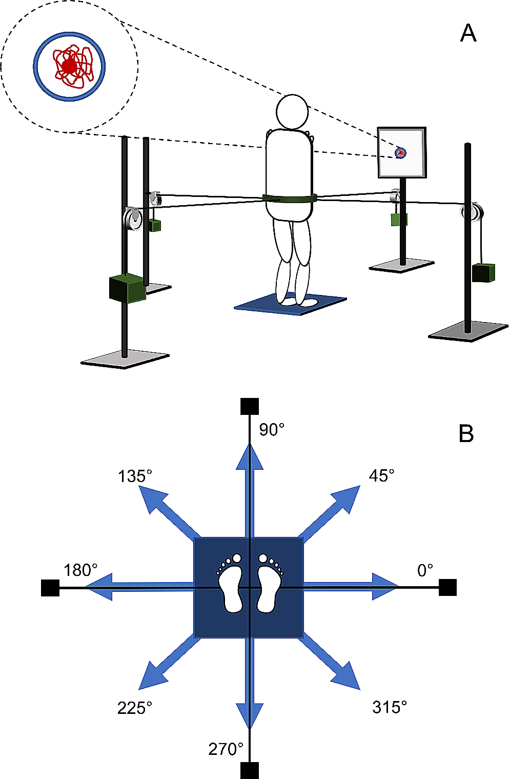
One single experimental session was conducted for each participant. They were asked to maintain their normal standing position on a force platform while looking at a monitor where real-time feedback of the 2-D position of their CoP was provided. The feedback was a red circular cursor of 0.5 cm diameter displayed on the monitor positioned 1.5 m in front of the subject (see Fig. 1-A) and with a refresh rate of 12 Hz. Participants positioned their hands at the level of the shoulders to avoid any contribution/assistance of the arms’ motion.

(A) experimental set-up rear view; (B) pulling forces directions. The participant stood on the platform with the hands positioned at the level of the shoulders while looking at the monitor where real-time feedback (represented by the dot) and the target (represented by the circle) were provided. After 5 s of standing position a pulling force (one of those reported in panel B) was applied

After 5 s of standing position, a pulling force of one of two different magnitudes (5% or 10% of body weight; BW) was applied at the level of the waist (Fig. 1-A) by means of a cable. To do that, an inelastic belt with four hooks was worn at the hip level. The hooks were attached to the belt, as reported in Fig. 1-A, and four different poles positioned in front, behind, to the left and right side of the subject with a pulley and a weight support were utilized for applying the pulling force. These specific loaded conditions were selected after several pilot experiments, where different loaded conditions were tested. These loads, expressed as percentages of the body weight, are indeed able to elicit significant variations of the EMG amplitude in the recruited muscles, avoiding angular changes in the lower limb joints.

As the pulling force was applied, participants were instructed to maintain the starting position by keeping the red circular cursor within a blue circular target 12.5 mm in radius without loss of balance. Loss of balance was defined as stepping with at least one foot during the application of the external force. The trial ended when cursor had remained in the target for at least 10 consecutive seconds (Fig. 1-A). Typical trial duration was 20 s (5 s of baseline within the target, 5 s to reach the target after perturbation, 10 s within the target while maintaining a static posture counteracting the load. After that, the load was removed. To counteract the load, participants were required to contract the muscles. However, they were not allowed to move their feet. As their posture did not change, an isometric force was generated by leg and trunk muscles.

The pulling force was applied in eight evenly spaced directions in the horizontal plane: 0°, 45°, 90°, 135°, 180°, 225°, 270° and 315° (where 0° corresponds to the right side of the participant; see Fig. 1-B for further details). Each direction was repeated 5 times with two load conditions: 5% BW (Light) and 10% BW (Heavy) of participant’s body weight (BW). A total of 80 trials were conducted from each subject in a randomized order. Randomization was conducted using a specific online software (Randomizer.com). The randomization was conducted across series (5 series x 2 load x 8 directions). Passive recovery was adopted to avoid fatigue between trials.

During each trial the CoP displacement and the Ground Reaction Forces (GRF) in the anteroposterior (CoPx, Fx) and mediolateral (CoPy, Fy) directions were recorded using a force platform (AMTI, USA, 90 × 90 cm, sampling frequency at 1000 Hz).

The EMG activity of 16 muscles was recorded (ZeroWire, Aurion, Italy, sampling at 1000 Hz) from the right side of each participant. The muscles included: rectus abdominis (RA), tensor fasciae latae (TFL), biceps femoris long head (BF), tibialis anterior (TA), semitendinosus (SMT), semimembranosus (SMB), rectus femoris (RF), peroneus (PER), medial gastrocnemius (GM), lateral gastrocnemius (GL), erector spinae (ES), external oblique (EOB), gluteus medius (GLT), vastus lateralis (VL), vastus medialis (VM), and soleus (SOL). In this experimental set-up we investigated only one side of the body, assuming a symmetric activation of the other sides in accordance with previous studies (Torres-Oviedo and Ting 2007, 2010; Kubo et al. 2017).

All instruments (EMG, CoP, GRF, and real-time biofeedback) were synchronized. For each trial a data matrix with 16 EMG channels, GRF, and CoP displacement as a function of time was obtained.

All data processing was performed using Matlab software (version 9.12, MathWorks, Natick, MA, USA), RStudio software (RStudio Inc., Version 1.4.1103, Boston, MA, USA) and SPSS software (version 16.0, IBM Corp., Armonk, NY, USA).

Each trial showed a loading phase (where the load was applied and the subject counteracted it), a steady-state phase (where the subject remained with the CoP inside the target for at least 10 s) and an unloading phase (where the load was removed). Since we were not interested in the transient phases (loading and unloading phases), the raw data were analyzed only in the steady-state phase by means of custom Matlab routines. The GRF and CoP data were filtered with a zero-phase-lag 4th order Butterworth low-pass filter with a cut-off frequency of 30 Hz to remove the effects of postural adjustment and signal fluctuations that are not related to physiological parameters (e.g., as in the case of behavioral noise). For each trial, the two-dimensional GRF (i.e. combined Fx and Fy components) was calculated and normalized by the participant’s BW to check the real force applied during the steady-state phase (nGRF). The mean value of the resultant force was calculated during the steady-state phase as an indicator of the trial quality.

The CoP data was analyzed frame-by-frame using a Euclidean distance approach after filtering. We calculated the point-by-point distance from the center of the target to the CoP coordinates (i.e., the center of the red cursor) as an indicator of performance. After that, the mean values of the Euclidean distances obtained during the steady-state phase were calculated. In this regard, we calculated the Error performed by the subject during the task as the ratio between the Euclidean distance (in millimeters) and the radius dimension (12.5 mm). Therefore, values larger and lower than 1 indicated that the participant was outside or inside the target, respectively. Trials were considered successful when the error was lower than 1 (one) (i.e., indicate that the participant remained within the target). The effects of loading conditions and direction of pulling forces on nGRF and Error were tested with a two-way repeated-measures ANOVA with fixed effect as Load (2 levels: 10% BW and 5% BW) and Direction (8 levels: 0º to 315º). Whenever the Mauchly’s test of sphericity was not satisfied, the Greenhouse–Geisser correction for the degrees of freedom was applied. Pairwise comparisons with Tukey corrections were used to explore significant effects.

Raw EMG data were high-pass filtered at 35 Hz, de-meaned, rectified, and low-pass filtered at 40 Hz (Ting and Macpherson 2005). The EMG data were further integrated over 10-ms intervals to reduce the size of the data set. Only data obtained in the steady-state phase were utilized for further analysis. The EMG values of each muscle during the steady-state phase was normalized to the maximum value across all loads and directions (Torres-Oviedo and Ting 2007, 2010; Berger and d’Avella 2014). Finally, the mean value was calculated.

The variations of the muscle patterns across the experimental conditions were analyzed by identifying muscle synergies from the mean EMG activity collected during the steady-state phase. For each participant we obtained a set of 80 vectors, each representing the average activity of all recorded muscles for each trial in one experimental condition (8 directions × 2 loads × 5 trials). We then used a nonnegative matrix factorization (NMF) algorithm (Lee and Seung 1999; Ting and Macpherson 2005; d’Avella and Bizzi 2005; Thresh et al. 2006) to decompose each one of these muscle activity vectors (m) as the combination of a unique set of N time-invariant synergies (wi) multiplied by condition-specific scaling activation coefficients (ci):

$$\varvec= \sum _^_ }_+}_$$

(1)

where em is an N-dimensional vector of muscle activation residuals. Different matrix factorization algorithms have been used for the identification of muscle synergies, assuming that the observed EMG data can be modeled as a linear combination of a small set of basis vectors (Tresch et al. 2006). To assess the potential bias towards the heavy load condition (10% BW), muscle synergies were additionally extracted by normalizing the EMG values to the maximum value of 5% and 10% BW separately.

The NMF decomposition technique assumes that each muscle activation pattern is decomposed in a linear combination of a few non-negative muscle synergies and non-negative synergy activation coefficients. A small set of muscle synergies states that representing muscle activity vectors (m) in terms of the vectors wi and scaling activation coefficients ci is lower-dimensional because it requires a lower number of values than the number of values of all elements of the m vectors. In particular, such linear decomposition technique states that over a large number of observations m the components wi remain fixed, but the scaling activation coefficients ci are allowed to change and are sufficient to account for all variations in the data measured across different motor task conditions.

To extract a set of synergies, the iterative decomposition algorithm was initialized with random values for synergies and coefficients, and it stopped when the reconstruction R2 value increased by < 10− 4. At each iteration the algorithm performed two steps: (1) it updated the synergies given the data and the coefficients; (2) it updated the coefficients given the synergies and the data. The extraction was repeated 40 times with random initial conditions and only the synergy set with the highest R2 was retained. Then, final number of synergies was selected as in d’Avella et al. (2006), according to the curve of the reconstruction R2 as a function of N (i.e., number of set of synergies extracted). The number of synergies at which the curve of R2 showed a change in slope, indicating that adding additional synergies did not significantly improve the accuracy of the reconstruction (Tresch et al. 2006; d’Avella et al. 2006; Ranaldi et al. 2021), was selected as the optimal number of synergies. In this regard, assuming that the R2 follows a straight line, it is possible to identify the value of N after which the R2 curve is essentially straight. Therefore, a series of linear regressions, firstly taking into account the entire R2 curve and progressively removing one synergy from the regression interval. The mean square residual errors of the different regressions was calculated and used a determinant for the synergy number. Indeed, the optimal number of synergies was obtained when the mean square error was lower than 10− 3.

We examined whether the muscle synergies extracted by our algorithm were influenced by any inherent bias built into the method by comparting the R2 value for the reconstruction of the real data with the extracted synergies and the R2 value for the reconstruction of structureless simulated data with synergies extracted from those simulated data. The generation of structureless data involved a process whereby the samples for each muscle were randomly reshuffled independently of the muscle activation data matrix (m). Consequently, the resultant simulated data exhibited the same muscle amplitude distribution as the real data, but each muscle amplitude was uncorrelated with all the others. This verification was achieved by comparing the R2 values obtained from reconstructing real data with the extracted synergies against those derived from reconstructing structureless simulated data. For each simulated dataset we repeated 100 synergy extraction runs with the same procedure used for the real data (d’Avella and Bizzi 2005; Borzelli et al. 2013).

The effects of loading conditions and direction of pulling forces on the activation coefficients were tested with a two-way repeated-measures ANOVA with fixed effect as Load (2 levels: 10% BW and 5% BW) and Direction (8 levels: 0º to 315º). The Greenhouse–Geisser correction for the degrees of freedom was applied in case the Mauchly’s test of sphericity was not satisfied. Pairwise comparisons with Tukey corrections were used to explore significant effects.

We characterized the directional tuning of the synergy amplitude coefficients with a cosine function (d’Avella et al. 2006, 2008). Briefly, for each participant, synergy and load; we performed a multiple linear regression (Matlab function “regress”) to fit the following model.

$$c\left(\theta \right) = _ + _cos\theta + _sin\theta$$

(2)

where q is the direction of the perturbation, c is the synergy amplitude coefficient, and β0 is an Offset parameter. We then computed the Amplitude, r:

and the preferred direction, θPD:

$$^= }^\left(_ / _\right)$$

(4)

and re-wrote Eq. 2 as a cosine tuning function:

$$c\left(\theta \right)= _+r \text\left(\theta - ^\right)$$

(5)

The goodness of the fit was quantified with the r2 value of the multiple linear regression, and its significance was tested with an F test. We also quantified the variability of the preferred direction (θPD) across conditions by computing its angular deviation (AngDev) (d’Avella et al. 2008), defined as the square root of 2(1 − q), where q is the length of the vector resulting from the sum of unit vectors directed as the preferred directions divided by the number of vectors (angular.deviation function, R-package ‘circular’).

To compare the synergies extracted from different participants, we grouped them using hierarchical clustering. We used the similarity between a pair of synergies (Sij), computed with the subset of muscle common to all participants, to define a distance measure (dij = 1 − Sij) (Matlab function “pdist”) with the “cosine” method. Then, we created a hierarchical cluster tree from all synergy pairs (Matlab function “linkage” with the “average” distance method, i.e. using as distance between two clusters the average distance between all pairs of objects across the two clusters). The cophenetic correlation coefficient was calculated to measure how accurately the tree represented the dissimilarities between observations (Matlab function “cophenet”). We partitioned the hierarchical tree with the minimum number of clusters for which there was no more than one synergy from the same participant in each cluster (Matlab function “cluster”) (d’Avella et al. 2006). As an alternative approach, we determined the number of clusters by identifying the largest vertical difference between nodes in the dendrogram from the hierarchical clustering and drew a horizontal line across the midpoint. Then, the optimal number of clusters was determined by counting the number of vertical lines intersecting with the horizontal line. Hereafter, we defined the clustered synergies as cW to differentiate them from the w that resulted from the NMF for each participant; accordingly, the corresponding grouped scaling activation coefficients were defined as cC.