Study design and population

This retrospective study focused on hospitalized patients, specifically involving a random selection of 981 individuals diagnosed with T2DM who were admitted to the Department of Endocrinology and Metabolic Diseases at the Affiliated Hospital of Zunyi Medical University and the data collection period spanned from March 2021 to March 2023.

Diagnostic criteria for T2DM were established according to the 1999 World Health Organization (WHO) criteria [8]. For the diagnosis of DKD and MAU, the study adhered to the diagnostic guidelines outlined in the Chinese Guidelines for Clinical Diagnosis and Treatment of DKD [3]. The study subjects were categorized based on their urinary albumin excretion rate (UAER). Specifically, individuals with T2DM exhibiting a UAER ranging from 30 to 300 mg/24 h were assigned to the MAU group (n = 333). In contrast, those with T2DM and a UAER less than 30 mg/24 h were classified into the DM group (n = 648).

Inclusion criteria: (1) Age ≥ 18 years; (2) T2DM patients.

Exclusion criteria: (1) diabetic ketoacidosis; (2) gestational diabetes mellitus and other special types of diabetes mellitus; (3) hyperglycaemic hyperosmolar state or severe and recurrent hypoglycaemic events in the past 3 months; (4) severe renal or hepatic malfunction, psychological illnesses, or a history of cancerous tumors; (5) renal injury due to other diseases.

Estimating the required sample size

This study adhered to the EPV (Events Per Variable) principle for determining the sample size of the predictive model, as outlined in the literature [9]. With 15 independent variables entered into the logistic regression analysis, and considering an estimated incidence of MAU in patients with T2DM ranging from 20–40% [10]—taking the midpoint of 30%—and factoring in a 10% attrition rate, the minimum required sample size for the predictive model modeling group in this study was calculated as follows:

$$ N=\frac\text\text\text\text\text \text\text \text\text\text\text\text\text\text\text\text\text\text \text\text\text\text\text\text\text\text\text \times 10}\text\text\text\text\text\text\text\text}\times \left(1+10\text\right)$$

The modeling group comprised 2/3 of the total sample size, and the validation group constituted the remaining 1/3. The minimum sample size for the validation group was determined to be N = 275 cases, resulting in a total minimum sample size of N = 825 cases. The final inclusion of 981 cases in this study exceeded the sample size requirement. All participants were randomly divided into a training set (687 cases) and a test set (294 cases) in a 7:3 ratio. The training set was utilized for model construction, while the test set was employed for model validation, ensuring a robust assessment of the predictive model’s performance.

Data extraction and clinical indicator measurements

The electronic medical record system within the hospital served as the primary data source, encompassing a comprehensive set of 36 candidate variables for predictive modeling. These variables were thoughtfully selected based on systematic meta-analysis and consultation with clinical care specialists and medical experts. The candidate variables were further classified into three distinct categories: socio-demographic characteristics, disease characteristics, and clinical biochemical indicators.

Socio-demographic characteristics

Gender.

Age.

Days in hospital.

Number of hospitalizations.

Residence.

Education level.

Smoking.

Drinking.

Systolic blood pressure (SBP).

Diastolic blood pressure (DBP).

Body mass index (BMI).

Disease characteristics

Diabetes duration.

Family history of diabetes.

Glucose-lowering regimen (oral hypoglycemic agents, insulin therapy).

Past medical history (hypertension, stroke).

Diabetic complications (diabetic peripheral neuropathy (DPN), diabetic retinopathy (DR), Diabetic peripheral vascular disease (DPVD)).

Clinical biochemical indicators

Glycated hemoglobin (HbA1c).

Fasting blood glucose (FBG).

Total cholesterol (TC).

Triacylglycerol (TG).

High-density lipoprotein cholesterol (HDL-C).

Low-density lipoprotein cholesterol (LDL-C).

Albumin (ALB).

Blood creatinine (Scr).

Uric acid (UA).

Urea nitrogen (BUN).

Serum C-peptide.

2-hour postprandial serum C-peptide.

Neutrophil-to-lymphocyte ratio (NLR).

Platelet-to-lymphocyte ratio (PLR).

Mean platelet volume (MPV).

Serum 25-hydroxyvitamin D (25(OH)D).

These variables collectively constitute a comprehensive dataset that captures socio-demographic, disease-related, and clinical biochemical aspects, offering a robust foundation for the predictive modeling undertaken in this study.

The BMI was calculated by dividing an individual’s weight by the square of their height, expressed in kilograms per square meter (kg/m2). For individuals with a history of hypertension or those diagnosed with hypertension during hospital admission, the diagnostic criteria outlined in the latest practice guidelines were followed [11]. Previous stroke history, whether ischemic or hemorrhagic, was also taken into consideration. The diagnosis of DR was established through clinical diagnosis and fundus photography. DPN was diagnosed based on the patient’s medical history, physical examination, and electromyography. DPVD was identified through clinical evaluation and the detection of vascular ultrasound abnormalities.

Upon admission, all patients underwent a fasting period of over 8 h overnight. Subsequently, 5 ml of venous blood was drawn from the elbow in the early morning of the following day, while patients remained in a fasted state. Various biochemical indicators were analyzed using specific methods:

FBG was measured by the hexokinase method. HbA1c was detected by the high-pressure liquid chromatography method.TC, TG, HDL-C, LDL-C, ALB, Scr, BUN, Uric Acid UA, and Serum C-peptides were analyzed by the Olympus (AU2700) automatic analyzer. Serum C-peptide 2 h after a meal, platelet count, neutrophils, and lymphocytes were detected using a hematology analyzer.MPV was determined using a hematology analyzer. 25(OH)D was detected by electrochemiluminescence (reagents were purchased from Roche, Germany).MAU was determined using the Coulter Beckman AU5421 Automatic Specific Protein Analyzer, employing immunoscattering turbidimetry and supporting reagents. These meticulous diagnostic and laboratory procedures ensured comprehensive and accurate data collection for the study.

Data pre-processing

Data sets containing more than 20% missing values were excluded from the analysis. For the remaining missing values, imputation was performed based on the type of variable: the mean or median was used for numeric variables, while the plurality method was applied for categorical variables.This approach ensured a robust analysis while accounting for any potential gaps in the dataset.Given that the dataset primarily consists of numerical variables with widely varying ranges, we implemented standardization on the training set using normalization techniques to ensure model accuracy. The same scaling was then applied to the test set for consistency.

Statistical analysis

Data processing and statistical analysis were conducted using IBM SPSS (version 29.0). In analyzing the factors influencing the occurrence of MAU in patients with T2DM, it was observed that none of the continuous variables followed a normal distribution. Therefore, between-group comparisons were conducted using the Mann-Whitney U test, with results expressed as M (P25, P75). Categorical information was presented as n (%), and between-group comparisons were performed using the chi-square (χ2) test. Additionally, hierarchical information was compared using the Kruskal-Wallis H test. A significance level of P < 0.05 was deemed statistically significant.

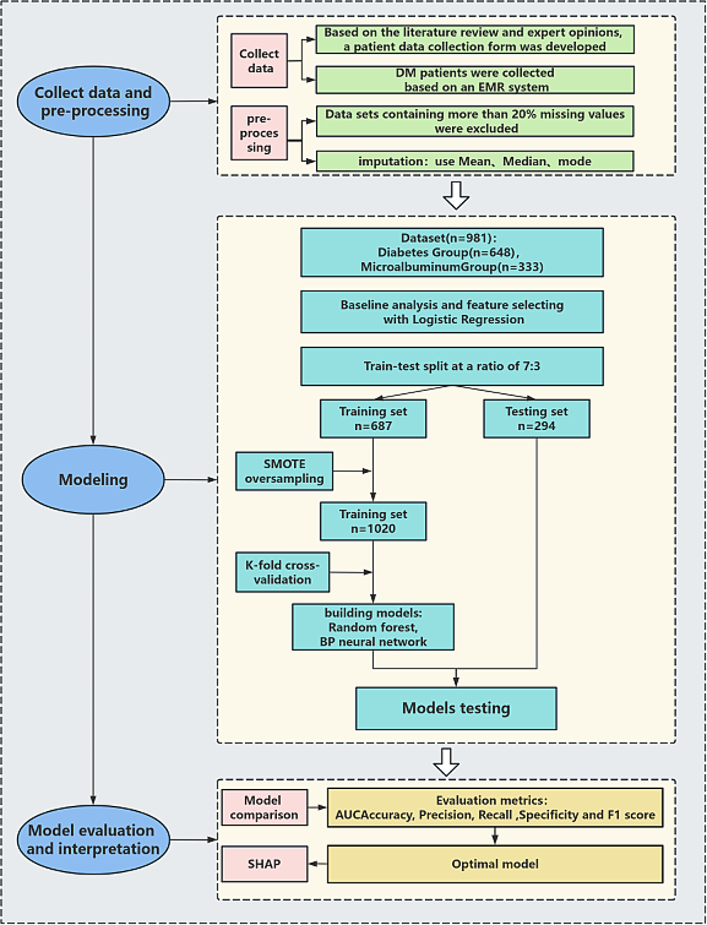
Model development

The risk prediction model was constructed using MATLAB software (version 2016b). The candidates for the prediction model underwent analysis through logistic regression. The independent variables identified through screening were then input into both Random Forest and BP neural network, respectively. The exact steps for building the prediction model in this study are outlined in Fig. 1.

The modeling process randomly divides the original dataset into a training set (70%) and a test set (30%), maintaining a balance of positive and negative samples. It’s worth noting that patient data in medicine often exhibit class imbalance, where general machine learning algorithms may favor predicting the majority class (usually samples) [12]. In this study, the dataset comprises 333 MAU patients and 648 MAU-negative patients. To address this data imbalance, we applied the Synthetic Minority Over-sampling Technique (SMOTE) [13] to the training data. Additionally, to mitigate randomness, the training set underwent cross-validation using the k-fold method (k = 5). This involves reserving one-fifth of the training set for testing, with the remaining four-fifths used for training iteratively. Model performance was evaluated using metrics such as the Area Under the ROC Curve (AUC), accuracy, precision, recall, specificity and F1 score. The average values of these metrics were calculated based on cross-validation.

Model interpretation

Effective model interpretation is crucial for clinical predictive models, and integrating interpretable machine learning algorithms enhances transparency and interpretability in clinical decision-making. In recent years, the SHAP method has emerged as a recognized tool for interpreting predictive models. SHAP is an algorithm designed to evaluate the contribution of multiple factors towards an outcome. This algorithm assigns weights to each feature in the model, calculating and ranking the influence of each feature on the outcome [14]. The SHAP model employs Shapley values to visualize the results of the predictive model in a SHAP plot.

Fig. 1

Establishment of a Forecasting Framework. SMOTE, Synthetic Minority Oversampling Technique, SHAP, Shapley Additive exPlanations