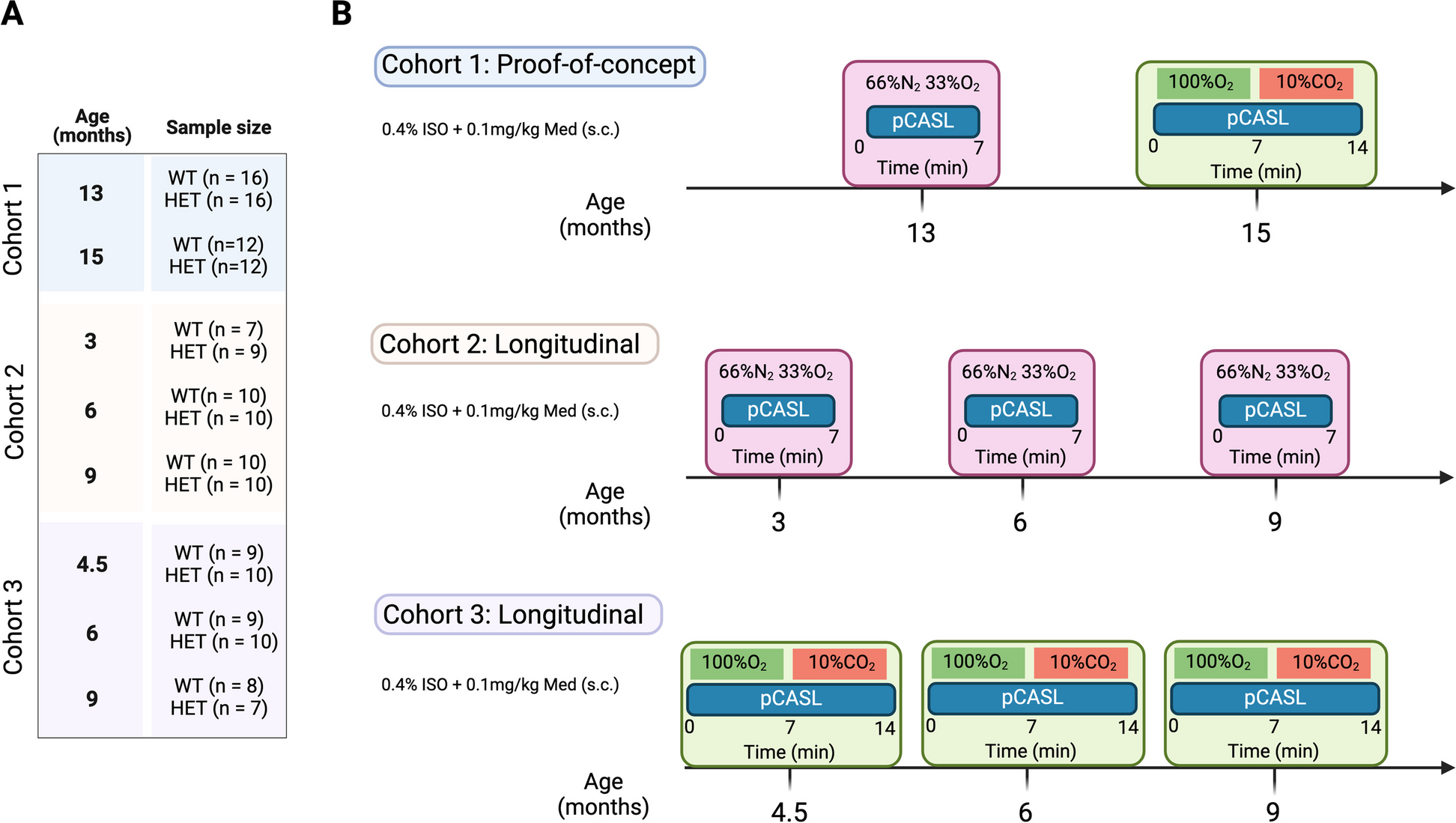
In this study, HET zQ175DN KI and WT [28] age-matched littermates (C57BL/6 J background, CHDI-81003019, JAX stock #029928), were used. The zQ175DN KI (without a floxed neomycin cassette) mouse model has the human HTT exon 1 substitute for the mouse Htt exon 1 with ~ 180–220 CAG repeats long tract. This model is a modified version of the zQ175 KI [23] where the congenic C57BL6J is used as the strain background [29]. The first motor deficits are observed at 6 months, marked as an onset of phenoconversion [22]. The HET form of zQ175DN has a slow progression reflected in the increase of mHTT aggregation from 3 until 12 months, initially appearing in the striatum at 3 and later in the cortex at 8 months of age [24]. A total of 36 HET zQ175DN KI and 35 WT age-matched littermates were used, distributed over 3 cohorts (Fig. 1A). We performed a proof-of-concept (PoC) study in cohort 1 for resting-state perfusion (13 months of age) and CVR (15 months of age), followed by two longitudinal pCASL studies where we assessed either resting-state perfusion or CVR: cohort 2 for resting-state perfusion (ages 3, 6 and 9 months of age) and cohort 3 for CVR (ages 4.5, 6 and 9 months of age (Fig. 1B). In all experiments, mice were initially anaesthetized with 2% isoflurane (Isoflo®, Abbot Laboratories Ltd., USA) in oxygen-enriched (66% N2 and 33% O2) for the plain perfusion studies [30], and for the CVR studies, 100% O2 during the baseline condition and 90% O2 + 10% CO2 [31] during the hypercapnic condition. The gas combinations were kept the same throughout the whole experiment. After the animal was positioned in the scanner, a subcutaneous bolus injection of medetomidine (0.05 mg/kg; Domitor, Pfizer, Karlsruhe, Germany) was applied followed by a gradual decrease of isoflurane to 0.4% over the course of 30 min which was kept at this level for the duration of the experiment. Meanwhile, a continuous subcutaneous infusion of medetomidine (0.1 mg/kg/h), starting 10 min post bolus medetomidine injection, was applied in combination with the isoflurane. The anaesthesia protocol used in this study is an established combination used for rodent resting-state fMRI [32, 33]. Throughout the experiment, all physiological parameters (breathing rate, heart rate, O2 saturation, and body temperature) were continuously monitored to ensure stable conditions. Animals were single-housed in individually ventilated cages with food and water ad libitum and continuous monitoring for temperature and humidity under a 12 h light/dark cycle. The animals were kept in the animal facility for at least a week to acclimatize to the current conditions before the experimental procedures.

Experimental design. (A) Sample sizes of WT and zQ175DN HET groups for each age and cohort (B) Experimental design for each cohort, for the proof-of-concept cohort 1, and the longitudinal studies: cohort 2 – resting-state CBF and cohort 3—CVR

MRI scans were acquired on a 7 T Pharmascan MR scanner with a 16 cm diameter horizontal bore, a quadrature 70 mm whole body resonator as a transmit coil and a 4 channel receive-only surface coil (Bruker, Germany). After positioning, three orthogonal T2-weighted Rapid Acquisition with Refocused Echoes (RARE) anatomical reference images (TR = 2000 ms, TE = 33 ms, matrix dimensions (MD) = (256 × 256), field of view (FOV) = (20 × 20) mm2, 12 slices) were acquired to enable a consistent slice package position for the pCASL scans for all subjects/time points. A time-of-flight angiogram was acquired to define the labelling position. Preceding the pCASL acquisition, two pre-scans were performed to optimize the phase of the pCASL label and control pulses [34]. The optimal label and control phases were subsequenlty used in all pCASL scans (i.e. in the perfusion scans of resting state and hypercapnic condition,, as well as in the labelling efficiency scan). Control and label images were acquired using the pCASL sequence [34] during which labelling pulses were applied in the neck (~ 8–11 mm caudal to the central imaging plane) with a duration of (\(\uptau )\) 3000 ms followed by a 200 ms post-labelling delay (PLD) and a single-shot spin echo planar imaging (SE-EPI) acquisition (TR = 3450 ms, TE = 19.5 ms, MD (96 × 64), FOV (25 × 25) mm2, spatial resolution (260 × 400) µm2, 5 slices of 0.8 mm slice thickness. To measure resting-state perfusion, 120 (60/60 control/label) images were acquired for 7 min. For the CVR, a baseline condition of 120 (60/60 control/label) images were acquired with a duration of 7 min, and from 7 until 14 min a CO2 challenge was administered and additional 120 images were acquired in that hypercapnic period (Fig. 1B). To calculate the labelling efficiency, α, a single (4 averages) label/control pCASL-scan with a flow compensated FLASH readout (labelling time of 200 ms without a PLD) is acquired, for one imaging slice located downstream the labelling plane, 4 mm caudal from the imaging volume. As the quantification of absolute CBF requires regional T1-values, additional non-selective inversion recovery (IR) scans were acquired with 23 inversion times (TI) ranging from 15 to 5000 ms and TR = 10 s, with identical SE-EPI parameters as the pCASL scan (total scan time 4 min 30 s). The total scan time for each experiment was approximately 1 h and 30 min.

T1 maps are calculated by the non-linear fitting of the T1-relaxation equation for inversion recovery: S(TI) = A + B exp(-TI/T1) to the signal intensities for the different TI, S(TI). Control and label images were realigned to the first scan, using a 6-parameter rigid-body spatial transformation estimated with the least-squares approach. Next, the individual IR image with TI = 5 s was co-registered to the mean image of the pCASL-scan, and the estimated transformation was applied to the T1 map. The absolute CBF-maps were calculated voxel-wise for each repetition (control/label pair of images) and slice, using the one-compartment model of Buxton [35] as shown in the following equation:

$$CBF=\frac__}}\right)}_^}}\cdot _\cdot \left(1-}\left(\frac_^}}}\right)\right)}$$

Here, \(\lambda\) is the blood–brain partition coefficient (0.89 ml/g), \(\Delta S\) is the magnetization difference (signal intensity) between control and label images using the surround subtraction method, \(__}\) is the T1 relaxation time constant of the arterial blood (1700 ms at 7 T), with α as the calculated labelling efficiency and T1’ the estimated T1 relaxation time constant. To account for variations in arterial transit time across multiple slices, effective PLD (PLDeff) was calculated, using an oscilloscope, given by the following equation:

$$PL_\left(slic_\right)=PLD+7ms+\left(slic_-1\right) x \frac$$

For the first slice, 7 ms needs to be added to the PLD because of a fat suppression gradient applied just before the image acquisition of this slice. The time remaining is then equally divided over the number of slices. To spatially normalize the CBF maps, we created a study-based EPI template from all subjects’ averaged EPI images for each time point in the PoC study and a 1st-time point-based template for each longitudinal study. Based on these estimated transformation parameters, all CBF repetitions per subject were normalized to the study-specific template. In-plane smoothing was applied to these normalized CBF maps using a Gaussian kernel with full width at half maximum of twice the voxel size. CBF maps were further averaged over repetitions per condition (baseline/CO2 challenge) to calculate the individual CVR, where % ΔCBF was obtained by using the following formula: ((CBFChallenge – CBFBaseline)/CBFBaseline) *100. Mice with bad labelling efficiency or T1 map were excluded from further analysis and the final sample sizes used are shown in Fig. 1A.

The above steps were performed using Statistical Parametric Mapping (SPM) using SPM12 (Wellcome Centre for Human Neuroimaging, London, UK). Template creation was done using Advanced Normalization Tools (ANTs).

Two types of analysis were performed to assess differences between genotypes in perfusion and CVR. First, an exploratory voxel-based (VBA) and second, a region-based analysis (RBA). For the RBA, parcels that encompass the region of interest (ROI) bilaterally, were manually delineated for each slice on the corresponding study-based template. The regions were based on previous studies in this model that have shown functional alterations [36, 37]. These included: retrosplenial cortex (RspCtx), cingulate cortex (CgCtx), somatosensory cortex 1/2 (S1/2Ctx), motor cortex 1/2 (M1/2Ctx), caudate putamen (CPu), piriform cortex (PiriCtx), insular cortex (InsCtx), thalamus (Thal), globus pallidus (GP), Visual cortex 1/2 (V1/2Ctx), auditory cortex (AuCtx) and claustrum (Cl), defined based on the Paxinos and Franklin’s mouse brain atlas, corresponding to 5 coronal Bregma levels: + 1.34 mm, + 0.26 mm, -0.46 mm, -1.82 mm and -2.30 mm. For each subject, at each age and condition, the mean CBF value for every region at different Bregma levels was extracted from the respective mean CBF map. Mean regional CVR values are extracted from the CVR map.

To assess blood vessel alterations, an IF study was performed on 60 age-matched, male WT (n = 6) and zQ175DN HET (n = 6) mice at 3, 6, 8,12 and 14 months of age for 8 brain regions: the Caudate putamen, medial (mCPu) and lateral portion (lCPu), CgCtx, InsCtx, PiriCtx, S1Ctx, M1Ctx and M2Ctx. Blood vessels were visualized with Lectin-Dylight 488 (1:25, Vector Laboratories, Cat. # DL-1174) and sections were imaged with a Perkin Elmer Ultraview Vox dual spinning disk confocal microscope, mounted on a Nikon Ti body using a 40 × dry objective (numerical aperture 0.95). Details regarding the brain preparation, IF protocol and imaging can be found in Vasilkovska et al [38].

A macro script was written for FIJI image analysis [39] and is available on github (https://github.com/DeVosLab/Huntington). Blood vessels were detected in maximum projections of 30 µm z-stacks. After background subtraction, a multi-scale tubeness filter [40] was applied to enhance both small and large vessel structures in the image. A user-defined threshold was used to segment the blood vessels in this enhanced image. The total area of these regions was quantified and reported as the projected blood vessel area. Skeletonization was performed on the obtained vessel masks after which the length of the main axis (defined as the longest path along the vessel) in the FOV was quantified. Data analysis was performed in R [41].

In the pCASL study, for the VBA, two-sample T-tests were performed to assess genotypic differences for each condition and each age (FDR corrected, p < 0.05, cluster size (k) ≥ 10). In the RBA, genotype differences were assessed for all ROIs per slice (multiple two-sample t-tests, FDR corrected, p < 0.05). In the longitudinal studies, to assess the temporal evolution of CBF and CVR changes for specific ROIs, a mixed effects model for repeated measures was applied with main factors of genotype and age and genotype*age interaction. In the case of interaction, post hoc comparisons (FDR corrected, p < 0.05) were performed for values within each genotype across ages compared to a control age of 3 months and between genotypes per age. When no interaction was present, the model was recalculated only for the main effects and a post hoc comparison (FDR, p < 0.05) was performed for each effect separately.

In the IF study, image-based outlier detection was applied using the median ± 3 × median absolute deviation as outer limits within each brain region and animal ID. If fewer than 3 images were retained, the animal ID was discarded from further analysis for the specific region. In the next step, all variables were averaged for each animal ID and region after which a similar, ID-based outlier detection was applied. For longitudinal assessment of all markers, two-way ANOVA was used with main factors of genotype and age and genotype*age interaction. In the case of an interaction, the same post hoc comparisons were applied as for the mixed effects model in the RBA analysis of the pCASL study. When no interaction was present, the model was recalculated only for the main effects and a post hoc comparison (FDR, p < 0.05) was performed for each effect separately (for age, comparisons are made to 3 months as a control). Outlier detection was performed in R. All statistical analyses and graph visualizations were performed using GraphPad Prism (version 9.4.1 for Windows, GraphPad Software, San Diego, California USA, www.graphpad.com).