
記住我
Hearing loss results in challenges with communication, which in turn may lead to social isolation, cognitive decline, and depression due to the lack of social interaction. The purpose of hearing aids is to compensate for hearing impairment. To do so, it is crucial that they are fitted in close accordance with the hearing abilities of the individual user. Hearing loss often develops over time, and this necessitates recurrent re-fitting of the hearing device to maintain optimal compensation for the hearing loss. Traditionally, fitting of hearing aids is carried out in the clinic and is based primarily on the estimation of frequency specific hearing thresholds in the form of an audiogram. The audiogram is used to set the gain of the hearing aid at different audiometric frequencies.
Traditionally, the audiogram is estimated based on behavioral tests, such as pure tone audiometry. Alternatively, hearing thresholds can be estimated from electrophysiological measures, such as the auditory steady-state response (ASSR) [1, 2]—neural activity evoked by amplitude- and/or frequency-modulated acoustic stimuli—which can be recorded from electroencephalography (EEG) electrodes placed on the scalp. Physiological hearing thresholds are found to be elevated 10–25 dB relative to behavioral hearing thresholds in normal hearing subjects and 5–20 dB in hearing impaired subjects depending on recording length [2–7]. This offset is consistent across studies and can therefore be taken into account in a fitting procedure. ASSR recordings are typically performed in the clinic and require dedicated equipment and trained personnel.
Over the last decade, a new EEG recording approach called ear-EEG has been developed [8, 9]. Here, EEG electrodes are placed in or around the ear, allowing the recording platform to be more discreet. Christensen et al have shown that it is possible to estimate physiological thresholds using ear-EEG in both normal hearing [10] and hearing-impaired subjects [11]. Combined with a mobile EEG recorder, ear-EEG allows for automatic and unsupervised estimation of hearing thresholds outside the clinic. Integrated into a hearing aid, this technology would therefore enable both initial and recurrent refitting of the hearing device in the daily life of a user.
The ASSR is of relatively small amplitude compared to background noise (spontaneous EEG, and other physiological and non-physiological sources). It is therefore necessary to average the EEG signal over relative long time in order to suppress noise and achieve a sufficiently high signal-to-noise ratio (SNR) [2]. Moreover, the same auditory stimulus shall be presented several times at different sound pressure levels (SPL) making ASSR-based hearing tests a time-consuming procedure. Using ideal experimental settings: performed in a quiet laboratory on sleepy/relaxed subjects, using chirp stimuli [12] and multiple band stimulation [13], several studies reported an average time of about 20–30 min for accurate physiological threshold estimation [14–17]. However, in real life settings, this time may be longer due to increased noise [18].
The traditional stimuli used in ASSR-based hearing tests, such as pure tones and chirps, are synthetic and monotone, and are therefore rather dull and unpleasant to listen to. The combination of long testing time and unpleasant synthetic stimuli makes them unsuitable for the everyday use case described above.
An ASSR-based fitting procedure outside the clinic must be more convenient than those currently used in clinical practice; the procedure should require as little effort and engagement from the user as possible and should be as imperceptible as possible. Accordingly, stimuli based on naturally occurring sounds would be more suitable.
Several studies have shown that there is neural entrainment to nonperiodic stimuli, such as speech and music [19–21]. The auditory cortex follows the envelope of speech and consistently reacts to changes in the envelope [22]. Laugesen et al [23] recorded ASSR to NB-chirps modified by imposing a speech envelope on the stimuli.
An alternative approach is to construct an ASSR stimulus where natural speech is used as a carrier signal. By applying an amplitude modulation to the speech signal, it is possible to create a sound stimulus that is able to evoke an ASSR. By filtering the speech signal into multiple frequency sub-bands and imposing the amplitude modulation to one or several of the frequency sub-bands (using different modulation frequencies), it is possible to stimulate a frequency specific ASSR. The stimulus can, in principle, be created in real-time based on the ambient sounds in the user's environment, thereby further increasing the feasibility of implementing a hearing test into daily life.
The amplitude of the ASSR depends on the intensity of the stimulus, i.e. ASSR increases with increasing SPL [1, 2, 24]. Natural occurring sounds, such as speech, vary in intensity over time and hence the intensity of each period of an amplitude-modulated (AM) speech signal also varies over time. Since the ASSR is an envelope-following response, the ASSR amplitude to AM speech stimulus will also vary over time. ASSR as a function of intensity can therefore be estimated by partitioning the recorded EEG signal according to the SPL of the corresponding AM speech stimulus. For accurate estimation it is crucial to compensate for the apparent latency of ASSR—the time between stimulus onset and ASSR onset [2].
In this study, we present an approach where the ASSR vs. presentation level relation can be estimated using a partly AM running speech signal. We show that this relation can be estimated both in scalp- and ear-EEG.
2.1. SubjectsTwenty-two subjects (11 women, average age 32.7 years (SD = 8)) participated in the study. All subjects had normal hearing (<20 dB HL for octave frequencies between 500 and 4000 Hz) and no history of hearing diseases. Behavioral hearing thresholds were measured for each ear using the ascending method described in ISO 8253-1:2010 [25].
Exclusion criteria were: known hearing loss, use of medications that stimulate the central nervous system, epilepsy or other brain disease. All test subjects gave written and informed consent before inclusion in the study. The study was approved by the Institutional Review Board at Aarhus University (no. 2021- 88).
2.2. Measurement setupEEG was recorded concurrently from four scalp electrodes and 12 ear electrodes. The scalp electrodes were placed at the left (M1) and right (M2) mastoids, Fpz and AFz, according to the 10–20 EEG electrode system, and attached to the skin using custom designed electrode holders made of silicone with double adhesive pads. Alcohol swabs were used to clean the skin prior to the attachment of the scalp electrodes. A small amount of gel (Electro-Gel, Electro-Cap International, Inc., USA) was applied on the scalp electrodes.
The 12 ear electrodes, six in each ear, were placed on individually designed earpieces in positions according to the labeling scheme for ear-EEG electrodes described by Kidmose et al [8]. For the current study, the following ear-electrode positions were used: ExA, ExB1, ExB2 and ExC in the concha part of the ear, ExJ in the ear-canal, and ExT located on the tragus, where x denotes the left (L) or right (R) ear (see figure 1).
Figure 1. Left: computer model of a left ear earpiece illustrating the position of the electrodes. Right: schematic illustration of the electrode configurations.
Download figure:
Standard image High-resolution imageThe earpieces were modeled based on individual ear casts using 3D software (EarMouldDesigner, 3Shape, Denmark) and made of biocompatible silicone (Detax softwear 2.0, Detax GmbH, Germany). Prior to insertion of the earpieces, the ears were cleaned with a water-soaked cotton swab.
The EEG recordings were acquired with a TMSi Refa16e EEG amplifier (TMSi, The Netherlands) with a sampling rate of 2500 Hz and an average reference. All recording electrodes were dry-contact Ag/AgCl electrodes with a diameter of 4 mm [26]. The ground electrode was placed on the neck using a disposable wet gel electrode (Ambu WS, Ambu A/S, Denmark). To maintain the active shielding provided by the amplifier, all electrodes were connected to the amplifier using coax cables.
Before the actual recordings, an initial check of the signal quality was performed by making a visual inspection of the signals in a live-viewer. The experimenter ensured that the signals resembled EEG and inspected for the presence of artifacts when the subject was instructed to perform eye blinks and facial muscle movements.
The auditory stimuli were presented to the test subjects using insert earphones (3 M E-A-RTONE for ABR, 50 Ohm, 3 M, USA) via an RME soundcard (Fireface UC, RME, Germany) with a sampling frequency of 48 kHz. The tubes from the earphones were inserted into the sound bore of the earpieces. The receiver was calibrated using an ear and cheek simulator (43AG, G.R.A.S. Sound and Vibration, Denmark) powered by a 12AA power module (G.R.A.S.) and a 42AA pistonphone (G.R.A.S.).
In order to synchronize the sound stimulus and the EEG data, a trig signal generated by the soundcard was fed to the trig input of the EEG amplifier via a trigger box (g.TRIGbox, g.tec medical engineering GmbH, Schiedlberg, Austria). The trig signal was generated by one of the audio channels of the soundcard, and the trig signal was periodic with a frequency of 0.1 Hz.
2.3. ASSR stimuli and recordingsTwo types of sound stimuli were used in the current study: white Gaussian noise (later white noise stimulus or WNS) and an audiobook narrated in english by a male narrator (later speech stimulus or SS). Silent pauses in the speech stimulus were truncated to 0.1 s.
Both stimuli were designed using the following steps:
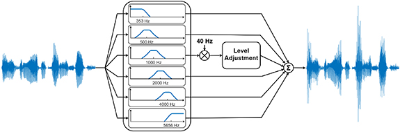
Figure 2. Schematic representation of the stimulus design.
Download figure:
Standard image High-resolution imageFigure 3. Illustration of the level adjustment procedure. The lower left panel shows the input distribution of the audio signal in the AM sub-band. The upper left panel shows the empirical level adjustment function, which transforms the continuous input distribution into the discrete output distribution. The upper right panel shows the amplitude distribution after the level adjustment.
Download figure:
Standard image High-resolution imageStimuli were generated in Matlab (R2020b, The Mathworks Inc., USA).
The objective was to impose an AM on a sub-band of the speech signal, as illustrated in figure 2. In order to estimate the ASSR as a function of the stimulus level, the AM sub-band of the speech signal was divided into short sub-segments, and each sub-segment was then assigned to one of the predefined levels. This was done by first calculating the RMS for each 50 ms sub-segment of the signal; and second, by means of an empirical amplitude transformation, scaling each sub-segment to one of the predefined levels. The empirical amplitude transformation was made such that more sub-segments were assigned to the lower levels, and fewer to the higher levels, so that the resulting noise level in the ASSR estimation followed approximately the shape of the ASSR, thereby maintaining an almost constant SNR across the different stimulation levels. The AM sub-band in SS contained 30, 24, 20, 20, 18, 18, 14, 12, 12 and 12 min at levels 0, 5, 10, 15, 20, 25, 30, 35, 40 and 45 dB SPL respectively (see figure 3).
The AM sub-band in the WNS contained 12 min at 45 dB SPL. The intention of using WNS was to create a reference stimulus that had design characteristics similar to SS (i.e. having an AM sub-band), but presented as a traditional steady-state stimulus.
The stimuli were presented monaurally relative to the behavioral hearing threshold (i.e. sensation level (SL)) at 1 kHz at the predefined levels as described in the stimulus design above. The stimulation side used was randomly chosen and evenly distributed across subjects. WNS was presented first, followed by SS.
The EEG recordings were performed in a double-walled, sound-attenuated room. The room was equipped with a window through which the experimenter was able to monitor the subject throughout the recording.
During the EEG recordings, the subjects were sitting in a comfortable chair. They were instructed to relax during the experiment but avoid falling asleep. They were offered to watch a silent movie of their own choice with subtitles.
2.4. Data analysis of EEGAnalysis of the EEG data was performed offline after the recordings were completed. ASSRs were estimated from three different electrode configurations: scalp-EEG, cross-ear-EEG and in-ear-EEG (see figure 1). For convenience, hereinafter we will refer to these three configurations as Scalp, CrossEar and InEar. Scalp datasets were created by re-referencing electrodes M1 and M2 to Afz (the Fpz electrode was included only as a backup in case of poor contact to the Afz electrode) for left and right side configurations, respectively. For both ear-EEG configurations, the datasets were created by applying a spatial filter, taking a weighted combination of the electrodes (for more details, see section 'Spatial filter for ear-EEG') thereby transforming multi-channel ear-EEG signals into a single-channel signal. For CrossEar, the spatial filter was applied to electrodes from both ears, resulting in one dataset for this configuration. For InEar, the spatial filter was applied to the electrodes from each ear individually, resulting in two datasets—one dataset for each ear.
For all configurations, the data was a band-pass-filtered using an 8th order, zero-phase filter with passband between 20 and 60 Hz and Butterworth characteristic. A notch filter was applied to remove 50 Hz line noise.
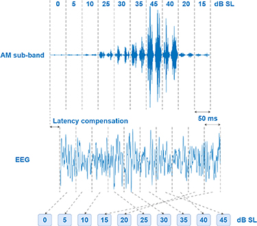
In order to align the recorded ASSR with the AM sub-band in SS, the EEG signal was shifted relative to the trigger signal by the required number of samples corresponding to the apparent latency (for more details, see section 'latency compensation'). The trigger signal was used to split the dataset into epochs of 10 s length. Each epoch was then split up into sub-epochs of 50 ms length. The sub-epochs were distributed among 10 datasets according to levels in the AM sub-band (see figure 4).
Figure 4. Schematic illustration of how EEG data was distributed among different levels. First, EEG data was aligned with the audio and then split up into 50 ms sub-epochs (corresponding to two periods of the modulation frequency). The sub-epochs were then distributed according to levels in the AM sub-band.
Download figure:
Standard image High-resolution imageWithin each dataset the sub-epochs were combined into four seconds epochs, which were then averaged using weighted averaging as described by John et al [27].
For ASSR recorded to WNS, the dataset was split up into epochs of four seconds length and the epochs were averaged using weighted averaging [27].
The averaged epoch was then transformed into the frequency domain by means of a discrete Fourier transform (DFT). The amplitude of the ASSR was determined as the amplitude at the modulation frequency bin, and the background noise was calculated as the RMS in the frequency band ±8 Hz relative to the modulation frequency (excluding the modulation frequency) [2].
Statistical significance of the ASSR amplitude was determined based on an F-test as described by Zurek [28]. The F-ratio was calculated as the ratio between the power at the modulation frequency and the average power in the frequency band ±8 Hz relative to the modulation frequency (excluding the modulation frequency). An F-ratio with a p-value ⩽ 0.05 was regarded as statistically significant. Only statistically significant ASSRs were included in the grand average across the subjects. Both ipsilateral (IL) ASSR (stimulation and recording from the same side) and contralateral (CL) ASSR (stimulation on one side and recording from the opposite side) were analyzed for Scalp and InEar configurations.
2.4.1. Latency compensationIn order to align the AM sub-band in the SS with the recorded EEG, it was necessary to estimate the apparent latency for the ASSR. The apparent latency can be estimated by calculating the cross-correlation between the analytic EEG signal  and the envelope of the AM sub-band signal
  .
.

where  represents the Hilbert transform operator.
To calculate the envelope  , AM sub-band
  was down-sampled to the EEG sampling frequency and the envelope was calculated as an amplitude of the complex-valued analytic signal
  . EEG data
  was epoched according to the trigger signal and epochs were combined again into one data segment. Both the envelope and the EEG were band-pass-filtered using an 8th order, zero-phase filter with passband between 20 and 60 Hz and Butterworth characteristic. A notch filter was applied to remove 50 Hz line noise in EEG.
Cross-correlation curves were averaged across subjects, and the lag with the maximum average cross-correlation was considered the ASSR latency.
2.4.2. Spatial filter for ear-EEGThe spatial filter for the ear-EEG data was found by maximizing the SNR. The optimal spatial filter can thus be expressed as  , where
  and
and  are the signal and noise covariance matrices respectively. The solution to this optimization problem can be found by applying the generalized eigenvalue decomposition to
  and
and  and the optimal spatial filter is then the eigenvector associated with the largest eigenvalue [29–31].
To calculate the covariance matrices, the EEG data was transformed into the frequency domain using DFT and point-wise multiplied by rectangular window functions. For  , the data was multiplied by a window, which preserved the frequency bins in the range of ±8 Hz centered at the modulation frequency (excluding the modulation frequency bin). For
  only the modulation frequency bin was preserved, whereas all other frequency bins were set to zero. The inverse Fourier transform was then applied to recover the time-domain band-pass-filtered signal. The covariance matrix,
  , was calculated as the normalized sum of the covariance matrices for each epoch of 4 s length multiplied by the weights estimated as in weighted averaging [27]. For better suppression of the noise in the modulation frequency bin, and thereby better signal estimation, covariance matrix
  was calculated based on the weighted averaged epoch. To mitigate numerical problems in the generalized eigenvalue decomposition, Ledoit–Wolf regularization was applied to each of the covariance matrices [32].
The spatial filter was estimated based on the entire 180 min EEG data recorded during SS presentation, i.e. before data segmentation to the different levels, and then applied to EEG data for each level as well as to EEG data from WNS presentation. The spatial filter was normalized to have a 2-norm equal to , which is the same as the 2-norm of a pair of electrodes.
Statistical analysis of the data was performed using mixed-effect models in R (lme4, version 1.1-26, Rstudio R-4.0.3) [33]. The statistical model included  (
( : continuous variable),
  (
( : continuous variable),
  (
( : continuous variable) and
  (
( : IL, CL) as fixed effects and
  as a random effect. The decision to include the fixed effect
  was made retrospectively after inspection of the data. This was done to allow the model to model a nonlinear dependency between stimulus level and response. In retrospect, this is pertinent, as there is no consensus in the literature regarding a linear association between ASSR amplitude and sound intensity. Some studies have reported a monotonically increasing ASSR with rising intensity [24, 34, 35], while other studies have reported saturation of ASSR [36–38].
Statistical significance of the different fixed effects was tested by model reduction based on a likelihood ratio test using the function anova() in R.
Difference between ASSR at 45 dB SL derived from two different types of stimuli (SS and WNS) was tested using a paired t-test.
All 22 included subjects completed the study. The average behavioral hearing thresholds across the subjects were 2.09 (SD = 6.42), 1.34 (SD = 5.26), 3.41 (SD = 6.85), and 1.18 (SD = 7.35) dB HL for 500, 1000, 2000, and 4000 Hz respectively.
3.1. LatencyThe average latencies for Scalp were estimated to be 43.6 and 42.4 ms for IL and CL respectively. For CrossEar the average latency was found at 22.4 ms and for InEar it was 26.4 (IL) and 20.4 (CL) ms. These latencies were used in the subsequent ASSR analysis for each configuration/measurement side. For more details about latency estimation, please refer to the supplementary material (figure S1).
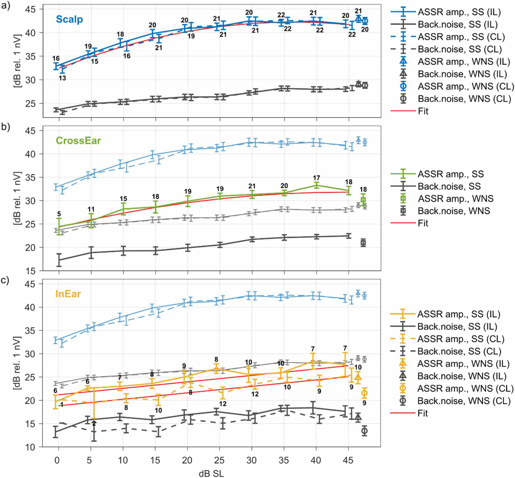
3.2. ASSR vs. dB SLFigure 5 shows the grand average ASSR and background noise as a function of dB SL derived from SS and WNS for the three different configurations: Scalp (a), CrossEar (b) and InEar (c). IL and CL measurements in Scalp and InEar are shown with solid and dashed lines respectively. The numbers above and below the error bars (standard error of mean) indicate the number of significant measurements in the grand average. Grand average for Scalp ASSR and background noise are plotted with faded colors together with both CrossEar (b) and InEar (c) for comparison. The estimated grand average ASSR and background noise values for the three configurations are included in table S1 in the supplementary material. Moreover, the ASSR and background noise figures for each individual subject are included in figures S2–S4 in the supplementaty material for Scalp, CrossEar and InEar respectively.
Figure 5. Grand average ASSR and background noise as a function of the dB SL for (a) Scalp, (b) CrossEar and (c) InEar configurations derived from SS and WNS. Error bars represent the standard error of mean. Solid and dashed lines in (a) and (c) represent IL and CL measurements respectively. The numbers above and below the error bars indicate the number of significant measurements included in the grand average. In (b) and (c) the grand average ASSR and background noise for Scalp configuration are presented in the background with faded colors to ease the comparison between the different configurations. The curves are shifted slightly horizontally for better readability. Red curves represent the fit from mixed models.
Download figure:
Standard image High-resolution imageA full mixed model was fitted to the measured ASSR amplitudes for each configuration. Visual inspection of the residuals did not reveal any obvious deviation from normality. Residual plots, Q-Q plots and histograms of the residuals along with model control analysis are included in the supplementary material (figures S5–S7). Model reduction tests are also included in the supplementary material (tables S2–S4). Coefficients of the final models, along with standard errors and 95% confidence intervals, are summarized in tables 1–3. The red lines in figure 5 show the fits from the mixed models.
Table 1. Fixed and random effect coefficients of the final model ASSR ∼ L + L2 + BT + (1|S) for Scalp.
Random effectsVarianceStd. Dev. Subject7.722.779 Residual4.142.034 Fixed effectsEstimateStd. Error95% Conf. Interval(Intercept)30.0311.114[27.86, 32.20]Level0.5390.028[0.48, 0.59]Level2−0.0070.0006[−0.0085, −0.0062]Behavioral threshold0.3040.112[0.085, 0.52]Table 2. Fixed and random effect coefficients of the final model ASSR ∼ L + L2 + (1|S) for CrossEar.
Random effectsVarianceStd. Dev. Subject13.663.969 Residual4.682.164 Fixed effectsEstimateStd. Error95% Conf. Interval(Intercept)24.3431.000[22.37, 26.31]Level0.3370.055[0.23, 0.44]Level2−0.0040.001[−0.0059, −0.0016]Table 3. Fixed and random effect coefficients of the final model ASSR ∼ L + MS + (1|S) for InEar.
Random effectsVarianceStd. Dev. Subject7.912.813 Residual6.452.539 Fixed effectsEstimateStd. Error95% Conf. Interval(Intercept)18.8420.820[17.23, 20.45]Level0.1380.018[0.10, 0.17]Measurement Side IL2.3520.431[1.51, 3.20]The ASSR amplitude increased with increasing presentation level for all electrode configurations (see figure 5). The likelihood ratio tests also revealed significance of the fixed effect  in all three configurations (Scalp:
  , CrossEar:
  , InEar:
  ). For CrossEar and InEar the ASSR amplitudes were approximately 10 dB and 15 dB lower compared to Scalp respectively. From figure 5 it appears that the slope of the ASSR amplitude is dependent on the presentation level. This was supported by the mixed model analysis, where the fixed effect
  was found to have significant effect for both Scalp (
 ) and CrossEar (
 ). For the Scalp configuration the slope of the ASSR amplitude was 0.42 dB/dB at 0–15 dB SL, 0.23 dB/dB at 15–30 dB SL, and practically 0 dB/dB at 30–45 dB SL. For CrossEar the slope of the ASSR amplitude curve was 0.26 dB/dB at 0–25 dB SL and 0.04 dB/dB at 30–45 dB SL. In contrast to Scalp and CrossEar, the curves for InEar were shallower and the fixed effect
  was not found to have significant effect (
 ). However, ASSR generally increased with increasing presentation level with a slope of 0.18 dB/dB.
The likelihood ratio test in the model reduction procedure for Scalp did not reveal the significance of  (
( ), which means no statistically significant difference between IL and CL measurements in Scalp. In contrast,
  was found to be significant for InEar (
 ). For InEar IL measurements were found to be significantly larger compared to CL measurements.
Analysis also showed that  was significant in Scalp (
 ) and nearly significant in InEar (
 ), but not in CrossEar (
 ). For Scalp the coefficient associated with the behavioral hearing threshold was 0.304 (see also table 1).
Statistical analysis did not show any differences between ASSR amplitude at 45 dB SL derived from SS and WNS (paired t-test,  for Scalp IL(CL);
  for CrossEar;
  for InEar IL/CL).
The estimated apparent latencies for Scalp EEG of 43.6 (IL) and 42.4 (CL) ms found in the current study are generally in good agreement with the latencies previously reported in the literature when taking the differences in stimulation level into account. Several studies reported an average apparent latency of 32–48 ms for ASSR with amplitude modulations of about 40 Hz [4, 34, 39–42].
The ASSR can be thought of as the summed activity of sources along the auditory pathway weighted by the individual source-electrode transfer function [1, 43]. In this regard, the quite long latencies found in the current study correspond to the latencies expected for activation of the auditory cortex [44], suggesting that cortex sources dominate the responses measured using the scalp configuration.
The latencies estimated for CrossEar and InEar EEG were shorter than those found for Scalp EEG. This indicates that sources earlier in the auditory pathway have a larger weight in the ear ASSR as compared to the conventional scalp ASSR.
4.2. Data segmentationAs part of the ASSR analysis, the EEG data was segmented into 50 ms long sub-epochs (two periods of the modulation frequency), which were sorted according to the intensity of the corresponding speech stimuli and recombined into ten level-dependent datasets. Recombination of the EEG data may introduce distortions into the EEG time series for every 50 ms, resulting in a 20 Hz artifact with a second harmonic at 40 Hz, which could interfere with the 40 Hz ASSR, leading to an increased false positive rate. To mitigate this, the EEG data was high-pass-filtered before the segmentation-recombination process. In order to investigate the effect of the high-pass filter, we compared the ASSR amplitude for the overall EEG data recorded to SS with and without random shuffling of 50 ms sub-epochs. For high-pass filters with cut-off frequencies above 10 Hz, the data segmentation-recombination did not change the amplitude at either 20 Hz or at 40 Hz in the periodogram of the EEG signal (see figure S8 in the supplementary material). Consequently, in the current study, a cut-off frequency of 20 Hz was used.
As an additional control, ASSR was recorded to WNS, that was designed in the same manner as the SS except that the level was held constant. WNS was therefore only presented at 45 dB SL, and the segmentation-recombination was not performed in the analysis of these data. The amplitude of ASSR recorded to WNS was comparable to the amplitude of ASSR recorded to SS at 45 dB SL and statistical analysis did not show any significant difference between ASSR derived from SS and WNS.
4.3. Spatial filterPrevious ear-EEG studies have shown that the ASSR SNR is lower fo
留言 (0)