ALS is a fatal disease involving death of motor neurons leading to progressive muscle weakness with eventual paralysis (Feldman et al., 2022). After frustrating decades of limited progress, tremendous steps have been made in recent years, yielding multiple new drug approvals, which has finally given clinicians a choice of medications to offer ALS patients (Mead et al., 2023). Previously, the only approved disease-modifying ALS treatments were riluzole (Bensimon et al., 1994) and non-invasive ventilation (Bourke et al., 2006). More recently, however, newly approved treatments have included edaravone (Edaravone MCI-186 ALS 19 Study Group, 2017), AMX0035 (sodium phenylbutyrate and taurursodiol) (Paganoni et al., 2020) and tofersen (for patients carrying SOD1 mutations) (Miller T. M. et al., 2022). Despite these milestones, ALS remains an incurable disease with many unanswered questions regarding upper and lower motor neuron failure and its underlying pathophysiology. Existing data has supported diverse pathomechanisms related to processes shared by other neurodegenerative conditions, which include defects in DNA/RNA, protein aggregation, proteostasis, neuronal networks, cytoskeleton structure, energy metabolism, inflammation and cell death pathways (Wilson et al., 2023). For all these processes, moreover, disease mechanisms are multilayered and influenced by specific genetic mutations, background disease-modifying genetic variants, environmental factors, and finally, by the ageing process itself (Akçimen et al., 2023). Increasingly, it has been appreciated that unraveling this complexity will require guidance from large-scale hypothesis-generating investigations that fully leverage multi-omics technologies (Morello et al., 2020). For this work, motor neurons, although a difficult cell type to isolate and study in humans, represent an epicenter of the ALS disease cascade and thus warrant special focus in efforts to understand disease mechanisms.

The evaluation of ALS motor neuron pathology has included studies of post-mortem CNS tissues as well as motor neurons differentiated from induced pluripotent stem cells (iPSCs) (Dimos et al., 2008). This latter approach has been implemented on a large scale as part of the Answer ALS project, which has now generated >1000 iPSC lines from ALS patients and controls along with transcriptome data from hundreds of these lineages (Workman et al., 2023). This approach offers the potential to obtain a functional genomic signature for ALS, based on motor neurons, using a much larger sample size than has been practical in post-mortem tissue studies. Results from this strategy, however, have been puzzling. An initial transcriptome comparison of 341 ALS and 92 control (CTL) iPSC lines from the Answer ALS project identified only 13 differentially expressed genes (DEGs) (Workman et al., 2023). Similarly, meta-analysis of 15 transcriptome datasets generated from iPSC-derived motor neurons identified only 43 genes differentially expressed between ALS (n = 323) and CTL (n = 106) samples (Ziff et al., 2023). Much larger numbers of differentially expressed genes, however, have been obtained from post-mortem tissue studies. A recent analysis, for example, used bulk tissue RNA-seq to compare post-mortem spinal cord segments between ALS (n = 154) and CTL subjects (n = 49), and identified 7349 and 4694 DEGs in the cervical and lumbar cord regions, respectively (FDR <0.05) (Humphrey et al., 2023). It is unclear why this degree of differential expression has not been replicated by iPSC transcriptome studies. On the one hand, bulk tissue RNA-seq may capture transcriptome changes stemming from multiple cell types, including microglia and astrocytes, leading to more profound differential expression (Yadav et al., 2023). Alternatively, iPSC-MNs may not be sufficiently differentiated to model the disease state of postmitotic motor neurons in ALS (Ho et al., 2016), leading to loss or diminution of in situ transcriptome differences that separate ALS from CTL motor neurons.

The application of laser capture microdissection (LCM) to post-mortem CNS tissue offers an approach for evaluating in situ motor neurons and their distinctive transcriptome signature in ALS patients (Jiang et al., 2005; Cox et al., 2010; Rabin et al., 2010; Kirby et al., 2011; Highley et al., 2014; Cooper-Knock et al., 2015; Ladd et al., 2017; Krach et al., 2018; Nizzardo et al., 2020). LCM allows RNA to be isolated from a motor neuron-enriched cellular pool, with less contribution from surrounding cell types as would occur with bulk tissue analysis (EmmertBuck et al., 1996). These studies have been informative but sample sizes have been limited and studies have varied with respect to laboratory methods, expression profiling platforms and statistical methods. Additionally, most analyses have focused on newly generated data only, without comparisons to previously published data. Conclusions have thus varied, although functional annotations of ALS dysregulated genes in LCM studies have related to cytoskeleton structure, RNA metabolism, RNA splicing and phosphatidylinositol-3 kinase signaling (Jiang et al., 2005; Cox et al., 2010; Rabin et al., 2010; Kirby et al., 2011; Highley et al., 2014; Cooper-Knock et al., 2015; Ladd et al., 2017; Krach et al., 2018; Nizzardo et al., 2020). There has been one meta-analysis study of three LCM-generated datasets comparing motor neuron expression between ALS and CTL samples, which identified 206 DEGs in common among datasets (p < 0.05, FC ≥ 2 or FC ≤ 0.50) (Lin et al., 2020). This study, however, did not include RNA-seq datasets, did not utilize a formal meta-analysis model, and only included studies of sporadic but not familial ALS patients.

This study reports findings from meta-analysis of six datasets in which LCM-dissected motor neurons were targeted for genome-wide expression profiling (Cox et al., 2010; Rabin et al., 2010; Kirby et al., 2011; Highley et al., 2014; Cooper-Knock et al., 2015; Krach et al., 2018; Nizzardo et al., 2020). The study incorporates both microarray and RNA-seq data and applies a random effects meta-analysis model to define differentially expressed genes (DEGs). The identified DEGs are compared to those linked to ALS by genome-wide association (GWA) studies as well as to genes altered in iPSC-derived motor neurons (Workman et al., 2023; Ziff et al., 2023) and bulk spinal cord segments (Humphrey et al., 2023). A novel approach utilizing nearest neighbor statistics is applied to identify putative transcription factor (TF) binding sites near DEGs and to further identify ALS-associated SNPs that may disrupt such sites. Results from this study define a high-confidence ALS transcriptome signature that provides a window into the in situ properties of motor neurons, cis regulatory mechanisms, and connections between ALS genetics and motor neuron biology.

Table 1 lists datasets incorporated into the meta-analysis. Preprocessing, normalization and differential expression analysis steps for each dataset are described below. All samples correspond to RNA pools from LCM-dissected lower motor neurons from post-mortem spinal cord segments. Prior to performing the meta-analysis, DEGs were identified with respect to each dataset individually using the same statistical thresholds (i.e., FDR <0.10 with FC > 1.50 or FC < 0.67).

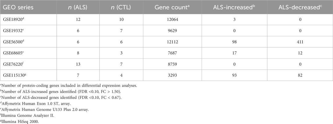
Table 1. Meta-analysis datasets. The table lists the 6 expression datasets incorporated into the meta-analysis. Sample sizes are listed for each dataset along with the number of genes included in each differential expression analysis. The final two columns list the number of differentially expressed genes identified with respect to each dataset individually. See footnotes for further details.

The dataset consisted of 22 samples from 12 sporadic ALS subjects (6 males, 6 females) and 10 CTL subjects (8 males, 2 females) (Rabin et al., 2010). The average age of ALS and CTL subjects was 66.4 (±3.2) and 72.8 (±3.3) years, respectively (Rabin et al., 2010). The average post-mortem sample collection interval was 4.4 (±0.33) and 5.1 (±1.05) hours for ALS and CTL subjects, respectively (Supplementary Figure S1A) (Rabin et al., 2010). RNA expression profiling was performed using the Affymetrix Human Exon 1.0 ST array platform. No prominent spatial artifacts were identified from microarray pseudo-images (Supplementary Figures S1B–W). Raw signal intensities had a similar distribution for each array, with the exception of CTL-1 (GSM468741), which had an increased frequency of low-intensity probes (Supplementary Figure S1X).

Quality control metrics were calculated using probe level models (PLM) (R package: oligo, function: fitProbeLevelModel) (McCall et al., 2011). PLM residuals were similar among arrays (Supplementary Figure S1Y). One sample (CTL-1) had a relatively increased normalized unscaled standard error (NUSE) median and interquartile range (Supplementary Figures S1Z, S1AA) (McCall et al., 2011). Likewise, CTL-1 had a relatively increased relative log expression (RLE) median (Supplementary Figure S1BB) although the RLE IQR was similar among arrays (Supplementary Figure S1CC) (McCall et al., 2011). Microarray normalization was performed using robust multichip average (RMA), including background subtraction, quantile normalization and median-polish summarization (R package oligo, function: rma) (Irizarry et al., 2003). RMA generated normalized intensity estimates for 22011 meta-probesets (MPS), of which 14303 could be unambiguously assigned to a single human gene symbol. In some cases, a human gene was represented by more than one MPS. The 14303 MPS were therefore filtered to include only one MPS per human gene, preferentially retaining the MPS for which mean RMA-normalized expression was highest across samples. This yielded 14141 MPS uniquely representing the same number of human genes, which were further filtered to include only 13611 MPS assigned to a protein-coding gene.

Since quality concerns were noted for CTL-1, MPS were excluded if expression of the CTL-1 sample was the highest or lowest among all samples, with a z-score-normalized expression estimate greater than 3 or less than −3. This yielded 13501 MPS. Of these, those with detectable expression in at least 15% of samples were retained (i.e., ≥4 of 22 samples), with detectable expression defined as an RMA-normalized expression value above the 15th percentile. This yielded 12064 MPS upon which differential expression analyses were based.

Linear models for differential expression analyses were estimated by generalized least squares using both sex and phenotype (ALS vs. CTL) as variables (R package: limma, function: lmFit) (Smyth, 2004). Sex was included in models since, as noted above, the proportion of males and females was dissimilar between ALS and CTL subjects. Moderated t-statistics were calculated using empirical Bayes shrinkage of the standard errors (R package: limma, function: eBayes) (Smyth, 2004). To control for multiple hypothesis testing among the 12064 MPS, raw p-values were FDR-corrected using the Benjamini-Hochberg method (Benjamini and Hochberg, 1995).

The dataset consisted of 13 samples from 6 ALS and 7 CTL subjects (Table 1). Of the 6 ALS samples, 3 were from subjects carrying CHMP2B mutations (Cox et al., 2010) while 3 were from subjects carrying SOD1 mutations (Kirby et al., 2011). For brevity, these data are referenced by the accession GSE19332 throughout this manuscript. However, CTL samples were submitted under two GEO accessions (GSE19332 and GSE20589), whereas samples for ALS patients with CHMP2B or SOD1 mutations are available under GSE19332 and GSE20589, respectively.

Gene expression was profiled using the Affymetrix Human Genome U133 Plus 2.0 array. Inspection of microarray pseudo-images did not reveal prominent spatial artifacts (Supplementary Figures S2A–M). Raw signal intensities showed good correspondence among samples (Supplementary Figure S2N). Probe-level model residual distributions were consistent among samples (Supplementary Figure S2O) (R package: oligo, function: fitProbeLevelModel) (McCall et al., 2011). Sample CTL-7 (GSM480310) had relatively elevated NUSE median and IQR values (Supplementary Figures S2O, P) but was otherwise unremarkable with respect to RLE median and IQR (Supplementary Figures S2R, S) (McCall et al., 2011). Expression summary scores for 54675 probe sets (PS) were calculated using RMA normalization (R package: affy, function: justRMA) (Irizarry et al., 2003). To limit redundancy (Li et al., 2008), a single PS was chosen to represent each human gene. To choose a representative PS, those PS with less specific probe sequences that may cross-hybridize with non-targeted transcripts (i.e., Affymetrix identifiers with an _x_ or _s_ suffix) were preferentially excluded. If there remained multiple PS after applying this criterion, the PS for which mean RMA-normalized expression was highest among the 13 samples was chosen as the representative.

The above steps yielded 20824 PS uniquely assigned to the same number of human genes, of which 17892 were assigned to a protein-coding gene. The MAS 5.0 algorithm was applied to determine which PS had detectable expression in each sample (R package: affy, function: mas5calls) (Liu et al., 2002). Differential expression testing was then performed using a subset of 9629 PS with detectable expression in at least 15% of samples (i.e., at least 2 of 13). Differential expression testing was performed as described above using general linear models and moderated t-statistics (R package: limma, functions: lmFit, eBayes) (Smyth, 2004). To correct for multiple hypothesis testing among the 9629 PS, raw p-values were FDR-corrected using the Benamini-Hochberg method (Benjamini and Hochberg, 1995).

The dataset consisted of 12 samples from 12 subjects, including 6 ALS subjects (4 males, 2 females) and 6 CTL subjects (5 males, 1 female) (Highley et al., 2014). The average age of ALS and CTL subjects was 60.2 (±3.5) and 61.7 (±3.9) years, respectively. Of the 6 ALS patients, 3 had sporadic disease and 3 carried C9ORF72 mutations. Expression profiling was performed using the Affymetrix Human Exon 1.0 ST array. Inspection of microarray pseduo-images did not reveal prominent spatial artifacts (Supplementary Figures S3A–L). Raw signal intensities differed among samples although no single sample emerged as an outlier (Supplementary Figure S3M). Likewise, the distribution of PLM residuals, NUSE median/IQR and RLE median/IQR did not identify any problematic samples (Supplementary Figures S3N–R).

Data normalization and processing steps mirrored those described above for GSE18920, which utilized the same microarray platform. RMA normalization was performed (R package oligo, function: rma) (Irizarry et al., 2003) and subsequent filtering steps yielded 13617 MPS uniquely corresponding to the same number of protein-coding human genes. Of these, 12112 MPS had detectable expression in at least 15% of the 12 samples (i.e., at least 2 of the 12 samples). Differential expression testing was performed on these 12112 MPS using generalized linear models with moderated t-statistics (R package: limma, functions: lmFit, eBayes). To correct for multiple hypothesis testing among the 12112 MPS, raw p-values were FDR-corrected using the Benjamini-Hochberg method (Benjamini and Hochberg, 1995).

The dataset included 11 samples from 8 ALS (3 males, 5 females) and 3 CTL (1 male, 2 females) subjects (Cooper-Knock et al., 2015). The average age of ALS and CTL samples was 62 (±1.5) and 60 (±4.0) years, respectively (Cooper-Knock et al., 2015). Expression profiling was performed using the Affymetrix Human Genome U133 Plus 2.0 array. Inspection of microarray pseudo-images revealed minor spatial artifacts for some samples, including CTL-1 (GSM1676861), CTL-2 (GSM1676862) and ALS-2 (GSM1676854) (Supplementary Figures S4A–K). However, raw signal intensity distributions were similar among samples (Supplementary Figure S4L) and no consistent outlier pattern was evident with respect to PLM residuals, NUSE median/IQR and RLE median/IQR (Supplementary Figures S4M–Q). Preprocessing and normalization steps were similar to those described above for GSE19332, which utilized the same array platform. RMA normalization generated signals for 17892 PS (R package: affy, function: justRMA) (Irizarry et al., 2003), of which 7687 had detectable expression in at least 15% of samples (i.e., at least 2 of 11 samples). Differential expression testing for these 7687 PS was performed using generalized linear models with moderated t-statistics (R package: limma, functions: lmFit, eBayes) (Smyth, 2004). To control for multiple hypothesis testing among the 7687 PS, raw p-values were FDR-adjusted using the Benjamini-Hochberg method (Benjamini and Hochberg, 1995).

The initial dataset consisted of 21 samples (Krach et al., 2018). However, fastq files downloaded for CTL-3 (GSM1977029) and CTL-8 (GSM1977034) were identical. The latter sample CTL-8 (GSM1977034) was therefore dropped from the analysis, after which there remained 20 samples from 13 ALS (9 males, 4 females) and 7 CTL (5 males, 2 females) subjects. The average age of ALS and CTL subjects was 63.3 (3.8) and 74.8 (2.8) years, respectively. The average post-mortem sample collection interval was 4.2 h (Supplementary Figure S5A) and the average RNA integrity number (RIN) was 5.7 (Supplementary Figure S5B).

Sequencing reads were generated using the Illumina Genome Analyzer II. Fastq file statistics were calculated using the FastQC software (Andrews, 2010). Prior to read filtering, there was an average of 28.7 million reads per sample, with no less than 11.3 million reads in any one sample (Supplementary Figure S5C). Read correction was performed using Rcorrector (Song and Florea, 2015) and adaptor and quality trimming was carried out using TrimGalore (Krueger, 2015). Sequences matching rRNA sequences were filtered out using the bbduk.sh shellscript contained within the BBTools software suite (Bushnell, 2018). Following these filtering steps, there was an average of 26.5 million reads per sample, with all samples having at least 10.4 million reads (Supplementary Figure S5D). Quality-filtered reads were mapped to the UCSC GRCh38/hg38 genome sequence using the STAR aligner (Dobin et al., 2013). Quantification of gene counts was performed with StringTie (Pertea et al., 2015). This protocol mapped 94.4% of reads on average (Supplementary Figure S5E), with 99.0% of reads on average assigned to intragenic sequence (Supplementary Figure S5F). An average of 87.1% of reads were assigned to exons (Supplementary Figure S5G) and only 0.4% of reads on average were assigned to ribosomal sequence (Supplementary Figure S5H).

Gene counts were generated for 18220 protein-coding genes. A gene was considered to have detectable expression if there was at least one mapped read and the Fragments Per Kilobase of transcript per Million mapped reads (FPKM) was greater than 0.3 (Ramsköld et al., 2009; Hart et al., 2013). Initially, analyses were performed on 10921 genes meeting these criteria for expression in at least 15% of samples (i.e., at least 3 of 20 samples; Supplementary Figure S6). However, inspection of MA plots revealed a relationship between FC estimates and gene abundance (Supplementary Figure S6D). This relationship was no longer apparent when the analysis was performed using 8759 genes with detectable expression in at least 50% of samples (i.e., at least 10 of 20 samples). This more stringent inclusion criteria was thus applied. For differential expression testing, raw gene counts were normalized using Trimmed Mean of M-values (TMM) (Robinson and Oshlack, 2010) and transformed to log-counts per million using the voom algorithm (Law et al., 2014) (R package: edgeR, functions: calcNormFactors, voom). Differential expression testing was then performed using precision weights estimated from the global mean-variance trend (Law et al., 2014), followed by fitting of generalized linear models and calculation of moderated t-statistics in a manner similar to that described above for microarray datasets (Smyth, 2004). To control for multiple hypothesis testing among the 8759 genes, raw p-values were FDR-corrected using the Benjamini-Hochberg algorithm (Benjamini and Hochberg, 1995).

The initial dataset consisted of 28 samples with sequencing reads generated from the Illumina HiSeq 2000 platform, which had been uploaded under three GEO series accessions (GSE115130, GSE76514, GSE93939) (Nichterwitz et al., 2016; Nizzardo et al., 2020). Throughout this manuscript, for brevity, only the GEO accession linked to ALS samples (GSE115130) is mentioned when referring to these data. The 28 samples included 10 from 7 ALS subjects and 18 from 10 CTL subjects. Of the 18 CTL, samples, there were six sample pairs for which fastq files were identical or nearly identical (GSM2027414:GSM3615509, GSM2027415:GSM3615511, GSM2027416:GSM3615501, GSM2027417:GSM3615503, GSM2027418:GSM3615504, GSM2027419:GSM3615505). Six of the duplicated samples were thus dropped from further analysis (GSM3615509, GSM3615511, GSM3615501, GSM3615503, GSM3615504, GSM3615505). This yielded a filtered dataset with 22 samples overall, including 10 ALS samples from 7 subjects and 12 CTL samples from 9 subjects.

There was an average of 6.6 million reads per sample prior to filtering (Supplementary Figure S7A). Read processing and filtering steps described above were applied, yielding an average of 4.8 million reads per sample (Supplementary Figure S5B). Quality-filtered reads were then mapped to the UCSC GRCh38/hg38 genome sequence using the STAR/StringTie pipeline described above (Dobin et al., 2013; Pertea et al., 2015). An average of 80.2% of reads were mapped (Supplementary Figure S7C), with an average of 97.1% of mapped reads assigned to intragenic sequence (Supplementary Figure S7D) and an average of 77.6% of mapped reads assigned to exonic sequence (Supplementary Figure S7E). Only 1.2% of reads on average mapped to ribosomal sequences (Supplementary Figure S7F). Nine samples were excluded from further analysis because the post-filter read count was less than 4 million reads, yielding 13 samples from 11 subjects. For cases in which more than one sample was available from the same subject, the sample with highest post-filter read count was retained. Following these steps, the dataset contained 7 ALS samples from unique subjects (GSM2465366, GSM2465372, GSM2465365, GSM2465370, GSM2465364, GSM2465363, GSM2465369) and 4 CTL samples from unique subjects (GSM3615508, GSM2027417, GSM2027419, GSM3615507).

Gene counts were quantified for 18220 protein-coding genes. Given that sequencing depth was limited, differential expression testing was performed for only 3293 genes with detectable expression in all 11 samples, where detectable expression was defined as indicated above (i.e., at least one mapped read with FPKM ≥0.30) (Ramsköld et al., 2009; Hart et al., 2013). Differential expression analysis was performed using the voom-limma approach described above (Law et al., 2014), and the Benjamini-Hochberg method was used to correct for multiple hypothesis testing among the 3293 genes (Benjamini and Hochberg, 1995).

Differential expression effect size was calculated based on the standardized mean difference (SMD) using the Hedge’s g estimator (R package: effsize, function: cohen.d) (Hedges, 1981; Hedges and Olkin, 2014). For microarray datasets (GSE18920, GSE19332, GSE56500, GSE68605), SMD was estimated using log2 scale RMA-normalized expression values (Irizarry et al., 2003). For RNA-seq datasets (GSE76220, GSE115130), SMD was estimated using TMM-normalized gene counts transformed to log2-counts per million (Robinson and Oshlack, 2010; Law et al., 2014), such that SMD estimates from both the array and RNA-seq datasets were calculated using a log2-based expression scale. SMD was only calculated for genes meeting the above-stated criteria for having detectable expression in a sufficient number of samples. If these criteria were not met for a given study, the overall SMD meta-estimate was based on fewer than 6 individual study estimates. Given this approach, an SMD meta-estimate was calculated for 9882 protein-coding genes for which at least 3 study-specific estimates were available (3 estimates for 2680 genes, 4 for 2776 genes, 5 for 2576 genes, and 6 for 1850 genes). Genes with 2 or fewer study-specific estimates were excluded from the meta-analysis. The SMD meta-estimate was calculated using a random effects meta-analysis model with inverse variance weighting (R package: meta, function: metacont) (Schwarzer, 2007). DEGs were identified based upon an FDR-adjusted p-value less than 0.10 with meta-SMD estimate greater than 0.80 or less than −0.80. The FDR threshold of <0.10 is consistent with prior transcriptome meta-analysis studies (Burguillo et al., 2010; Huan et al., 2016; Vora et al., 2018; Medina et al., 2023). The meta-SMD threshold of ±0.80 has been viewed as representing a “large” treatment effect in meta-analysis studies (Cohen, 2013), with SMD values exceeding 0.80 in absolute value corresponding to 53% or less overlap between two comparison groups (Andrade, 2020).

ALS-increased and -decreased DEGs were evaluated to assess for overrepresentation of annotations related to processes, functions, cell components or pathways (Maleki et al., 2020). The “universe” of background genes in all analyses was limited to the 9882 motor neuron-expressed protein-coding genes included in the meta-analysis. Enrichment of Gene Ontology (GO) biological process (BP), molecular function (MF) and cell component (CC) terms was assessed using a conditional hypergeometric test (R package: Gestates; function: hyperGTest) (Falcon and Gentleman, 2007). Fisher’s exact test was used to evaluate for enrichment with respect to terms from the Kyoto Encyclopedia of Genes and Genomes (KEGG) (Kanehisa et al., 2016), WikiPathways (Agrawal et al., 2024), Reactome (Fabregat et al., 2018), Disease Ontology (DO) (Kibbe et al., 2015), Pathway Commons (Rodchenkov et al., 2020), Medical Subject Headings (MeSH) (Yu, 2018), Drug Signatures Database (DSigDB) (Yoo et al., 2015), Molecular Signatures Database (MSigDB) (Liberzon et al., 2015) databases (R packages clusterProfiler (Yu et al., 2012), ReactomePA (Yu and He, 2016), DOSE (Yu et al., 2015), paxtoolsr (Luna et al., 2016), meshes (Yu, 2018) and msigdbr (Dolgalev, 2022)). Fisher’s exact test was also used to determine if any non-coding RNA targets were enriched among DEGs, based on ncRNA-target associations provided by the LncRNA2Target (Cheng et al., 2019), miRTarBase (Chou et al., 2018), miRDB (Chen and Wang, 2020) and TargetScan (Agarwal et al., 2015; McGeary et al., 2019). Likewise, Fisher’s exact test was used to identify protein interaction partners frequently interacting with mRNAs linked to DEGs, based on RNAInter database annotations (Kang et al., 2022).

Networks were generated to illustrate topological relationships among GO BP terms enriched with respect to ALS-increased and -decreased DEGs, respectively. In each case, the network was generated by drawing connections between enriched GO BP terms for which associated genes overlapped by at least 50% (R package: igraph) (Csardi and Nepusz, 2006). Groups of similar enriched GO BP terms were identified to color-code the network based on broader GO categorizations, with GO BP term groups identified using hierarchical cluster analysis with Euclidean distance and average linkage. For this analysis, the distance between two GO BP terms A and B was calculated using the distance metric 1—max (pA, pB), where pA and pB represent the proportions of overlapping genes associated with terms A and B, respectively. Groups of similar GO BP terms associated with overlapping gene sets were then defined based on the resulting dendrogram using variable height branch pruning (R package: dynamicTreeCut; function: cutreeDynamicTree) (Langfelder et al., 2008).

Protein-protein interactions were obtained from the STRING database (version 12.0) (Szklarczyk et al., 2023). Only high-confidence protein interactions were considered (confidence score ≥0.700). Of the 1850 genes having detectable expression in each of the 6 meta-analysis datasets, 1343 were linked to a protein having at least one high-confidence STRING database interaction, with an overall total of 4449 interactions among the 1343 proteins. The 1343 proteins were assigned to 12 subgroups based on average linkage hierarchical clustering (Euclidean distance), using a distance matrix with entries calculated from the confidence score between protein pairs (i.e., 1—confidence score) (R package: dynamicTreeCut, function: cutreeDynamicTree) (Langfelder et al., 2008). The dominant functional theme for each protein group was determined based upon the most significant GO BP term overrepresented in each group (R package: GOstats) (Falcon and Gentleman, 2007). The Kamada-Kawai algorithm was used to generate the protein-protein interaction network layout (R package: igraph, function: layout_with_kk) (Kamada and Kawai, 1989; Csardi and Nepusz, 2006). Network vertices and edges were color-coded based upon protein subgroup or SMD estimate.

Motif analyses were performed using the Jaspar Core vertebrate collection, consisting of 841 non-redundant experimentally-determined TF binding sites (Rauluseviciute et al., 2023). The 841 position frequency matrices (PFMs) were converted to position probability matrices (PPMs) using a pseudocount of 0.8 (Nishida et al., 2009). Genome analyses were performed using the telomere-to-telomere (T2T-CHM13) human genome sequence with annotated sequence coordinates for 19969 protein-coding genes (Nurk et al., 2022). The T2T genome sequence was used for motif analysis because it corrects assembly gaps from the GRCh38 genome, providing an additional 200 million base pairs with improved accuracy and coverage of complex repetitive genomic regions (Nurk et al., 2022). For each T2T-CHM13 chromosome, PPMs were converted to position weight matrices (PWMs) based on background nucleotide frequencies calculated for that chromosome (Wasserman and Sandelin, 2004). The chromosome sequence was scanned for PWM matches using a multinomial model with Dirichlet conjugate prior (R package: Biostrings, function: matchPWM) (Wasserman and Sandelin, 2004). Background nucleotide frequencies were calculated for each chromosome separately. A PWM model was considered to match a given locus if the correspondence score exceeded 80% of the theoretical PWM maximum score (Wasserman and Sandelin, 2004). Further analyses were performed on 798 motifs having at least one PWM match to each chromosome.

Transcription factors can regulate gene expression through binding at enhancer sites located far from target genes, with regulatory interactions spanning distances extending far beyond the upstream windows of 1 kb, 2 kb or 5 kb often recognized as gene promoter regions (Shlyueva et al., 2014; Chen et al., 2020). The current study therefore used a threshold-free nearest neighbor statistic to test for associations between PWM match locations and DEG transcription start sites (TSSs). For each PWM model and each protein-coding gene, the nearest neighbor (NN) distance was calculated, defined as the distance between the gene’s TSS and the closest PWM match on the chromosome. For these calculations, the most downstream TSS was used for genes associated with multiple isoforms with alternative TSS locations. NN distances among genes approximated a Poisson distribution for each PWM model. The distance ratio was defined as NNFG/NNBG, where NNFG represents the average NN distance among foreground genes (i.e., DEGs), and NNBG represents the average NN distance among background genes (i.e., all other genes included in the meta-analysis). A ratio less than one indicates that a PWM model has genome matches closer on average to the TSS of foreground genes. To evaluate the significance of this ratio, log10-transformed NN distances were compared between foreground and background genes using Welch’s two-sample two-tailed t-test (R function: t.test). To correct for multiple hypothesis testing among the 798 motifs, raw p-values were FDR-corrected using the Benjamini-Hochberg method (Benjamini and Hochberg, 1995). ALS-associated PWMs (AAPs) were defined as PWM models for which the average NN distance between genomic match locations and FG gene TSSs is lower (FDR <0.10) than that of BG gene TSSs.

SNP loci previously associated with ALS by genome-wide association (GWA) studies were identified from the NHGRI-EBI GWAS catalog (file: All associations v1.0) (Sollis et al., 2023). SNP loci were identified based on 7 catalog traits, including “ALS,” “ALS (age of onset),” “ALS (C9orf72 mutation interaction),” “ALS (sporadic),” “ALS in C9orf72 mutation negative individuals,” “ALS in C9orf72 mutation positive individuals” and “Rapid functional decline in sporadic ALS.” There were 175 unique SNPs associated with these traits, which were together associated with 323 genes based on reported, mapped, upstream and downstream catalog genes. Based on the 175 SNPs, a broader set of 2639 SNPs was identified by including those in linkage disequilibrium with the initial set of 175 (R2 ≥ 0.90) (R package: LDlinkR, function: LDproxy) (Myers et al., 2020). For each SNP, the nearest human gene was identified, leading to an additional 60 ALS-associated genes for an overall total of 383. Of these 383 genes, 204 were protein-coding motor neuron-expressed genes included in the meta-analysis. The location of each SNP was evaluated to determine if it was within an enhancer region, based on annotations available from GeneHancer (Fishilevich et al., 2017), the ENCODE Project (Consortium, 2012) and ORegAnno (Lesurf et al., 2016). Both alleles of each SNP were evaluated to determine if there was differential correspondence to any of the PWM models described above. A genotype-dependent PWM match was defined as one for which the correspondence score at a SNP-overlying locus exceeded 80% of the theoretical maximum score of that PWM for one allele but not the other (R package: Biostrings, function: matchPWM) (Swindell et al., 2015).

Expression changes seen in ALS patient motor neurons were compared to those in LCM-dissected motor neurons from SOD1-G93A mice (Gurney et al., 1994). Two datasets were evaluated (GSE10953 and GSE46298). The first (GSE10953) compared G93A to CTL mice on the C57BL6/J background at three time points, corresponding to presymptomatic (day 60), symptomatic (day 90) and late (day 120) stages of disease progression (n = 3 for each treatment/time combination) (Ferraiuolo et al., 2007). The second (GSE46298) evaluated mice from two strains (C57BL6/J and 129Sv), with comparisons between G93A and CTL mice at 4 time points corresponding to presymptomatic (day 56), onset (C57: day 133, 129Sv: day 101), symptomatic (C57: day 152, 129Sv: day 111) and endstage disease (C57: day 160, 129Sv: day 121) (n = 4 for each treatment/time/strain combination) (Nardo et al., 2013).

The GSE10953 dataset was generated using the Affymetrix Mouse Expression 430A array platform. Raw CEL files were normalized using the RMA algorithm (R library: affy, function: justRMA) (Irizarry et al., 2003) yielding signals for 22690 PS representing 13091 unique genes, of which 12765 were protein-coding. Of these, a subset of 11223 genes could be uniquely matched to a human orthologue based upon homology information from the Mouse Genome Database (Blake et al., 2021). Inspection of microarray pseudoimages revealed minor spatial artifacts on two arrays (Supplementary Figures S8Q, R) and these same arrays differed with respect to their raw intensity distributions and some quality-control metrics (Supplementary Figures S8S–X). However, none of the 11223 genes with human orthologues had outlying expression values for these two array samples (i.e., |z-score| < 3 for all genes). Additionally, no single array emerged as an outlier on cluster and PC analyses (Supplementary Figures S9A, D). There was minimal separation between G93A and CTL samples on cluster and PC analyses (Supplementary Figures S9A, D), although G93A and CTL samples did differ significantly with respect to the third PC axis (p < 0.05, two-sample two-tailed t-test; Supplementary Figure S9G).

The GSE46298 dataset was generated using the Affymetrix Mouse Genome 430 2.0 array platform. RMA normalization as above yielded signals for 45101 PS corresponding to 20493 unique mouse genes of which 17292 were protein-coding. Of the 17292 protein-coding genes, 14741 were uniquely matched to a human orthologue (Mouse Genome Database) and thus included in further analyses. No prominent spatial artifacts were detected on microarray pseudoimages and quality-control metrics were within an acceptable range for all microarray samples (Supplementary Figures S10, 11). For both strains, there was good separation between G93A and CTL samples in cluster and PC analyses (Supplementary Figures S9B, C, E, F) and there was a significant difference between G93A and CTL samples with respect to the first and/or second PC axis (p < 0.05, two-sample two-tailed t-test; Supplementary Figures S9H, I).

Differential expression testing (G93A vs. CTL) was performed as described above using general linear models and moderated t-statistics (R package: limma, functions: lmFit, eBayes) (Smyth, 2004). Testing was performed only for those protein-coding genes having human orthologues and detectable expression in at least one of the 6–8 samples involved in each comparison. Genes with detectable expression were defined as above based upon the Mas 5.0 algorithm (Liu et al., 2002) (R library: affy, function: mas5calls). Raw p-values were adjusted for multiple hypothesis testing using the Benjamini-Hochberg method (Benjamini and Hochberg, 1995).

Cell type-specific expression of genes was evaluated using single-nucleus RNA-sequencing data from post-mortem human lumbar spinal cord sections (GSE190442; n = 7 donors) (Yadav et al., 2023). Analyses were performed using QC-processed counts provided by Gene Expression Omnibus (file: GSE190442_aggregated_counts_postqc.csv.gz). Counts were obtained for 55289 cells from 64 cellular subtypes broadly classified into 11 categories (neurons, astrocytes, microglia, oligodendrocytes (OD), oligodendrocyte precursor cells (OPCs), Schwann cells, pericytes, endothelial cells, meninges, lymphocytes and ependymal cells). Raw counts were normalized to count per million mapped reads (CPM) and further analyses were performed using Log10(CPM +1) as an expression metric (Yadav et al., 2023).

Gene expression changes during motor neuron differentiation were evaluated using RNA-seq data from a time series in which in vitro monolayer human embryonic stem cells were differentiated to motor neurons (GSE140747; n = 45 samples) (Rayon et al., 2020). Retinoic acid and a smoothened (SMO) protein (hedgehog pathway component) agonist were used as differentiation-promoting agents. Raw sequencing reads were mapped to the UCSC GRCh38/hg38 genome using the STAR/StringTie pipeline described above (Dobin et al., 2013; Pertea et al., 2015). There was an average of 36.3 million quality-filtered reads among the 45 samples and the percentage of mapped reads, intragenic reads and exonic reads was greater than 90% for all samples (Supplementary Figures S12A–E). Cluster and principal component analyses demonstrated a strong time series effect without outliers (Supplementary Figures S12F, G). Changes in gene expression over time were evaluated using least-squares regression using voom-normalized expression data (Law et al., 2014), with FDR correction of raw p-values performed using the Benjamini-Hochberg approach (Benjamini and Hochberg, 1995).

The analysis incorporated samples from six datasets (Table 1). Cluster analysis showed better separation of ALS and CTL samples for two datasets (GSE68605 and GSE115130) compared to the other four (Supplementary Figures S13A–F). When samples were plotted in two-dimensional principal component (PC) space, however, there was stronger separation between ALS and CTL samples, such that linear discriminant functions classified disease status with accuracy ranging from 70% (GSE76220) to 100% (GSE68605) (Supplementary Figures S13G–L). For all datasets except GSE115130, ALS and CTL samples differed significantly with respect to at least one of the top 10 PC axes (p < 0.05, two-sample two-tailed t-test; Supplementary Figures S13M–R).

Goodness-of-fit testing based on model deviance was used to evaluate the contribution of other factors to gene expression variation (e.g., age and sex). This analysis was not performed for two datasets (GSE19332 and GSE115130) since disease status was the only annotation available. For GSE56500 and GSE68605, most gene expression variation was explained by disease status, which represented the dominant factor for 49%–56% of protein-coding genes (Supplementary Figures S14C–F). For GSE18920 and GSE76220, goodness-of-fit was similarly improved by disease status, sex, age and RNA integrity number (RIN), although disease status remained the dominant factor for 28%–30% of protein-coding genes (Supplementary Figures S14A,B, G–H).

Differential expression testing generated L-shaped raw p-value distributions reflecting an overabundance of low p-values (Supplementary Figures S15A–F). Consistent with this, t-statistic Q-Q plots were non-linear to support significant expression differences between ALS and CTL samples (Supplementary Figures S15G–L). Volcano plots demonstrated balanced FC estimates between ALS-increased and -decreased genes (Supplementary Figures S15M–R) and MA plots did not show FC differences between low- and high-expressed genes (Supplementary Figures S15S–X). There were 175 and 509 DEGs identified with respect to GSE115130 and GSE56500, respectively, although fewer DEGs (≤29) were identified in other datasets at the same significance thresholds (i.e., FDR <0.10, FC > 1.50 or FC < 0.67; see Table 1).

The number of protein-coding genes with detectable expression varied from 3293 to 12112 among datasets (Table 1). Among 1850 protein-coding genes with detectable expression in all six datasets, SMD estimates were positively correlated among four datasets (GSE68605, GSE56500, GSE76220, GSE189200), with estimates from these four datasets weakly correlated with those from the other two (GSE19332, GSE115130) (Figures 1A,B). SMD correlations ranged from −0.22 to 0.54 among 15 possible dataset comparisons (Figure 1B). Consistent with this, self-organizing maps color-coded by SMD estimates revealed regions with shared as well as dataset-specific patterns (Figures 1C,D). The 1850 protein-coding genes were associated with 1343 proteins having at least one high-confidence protein-protein interaction (PPI), with a total of 4449 interactions among the 1343 proteins (Figure 1E). The pattern of up- and downregulation varied across the PPI network with uniquely downregulated (GSE56500) and upregulated (GSE115130) components (Figure 1F).

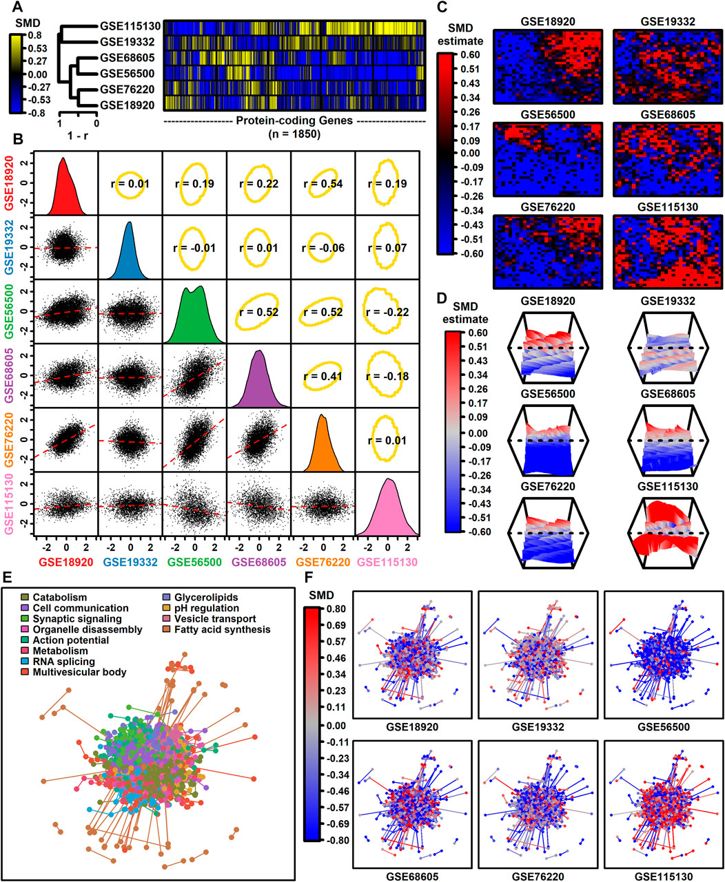
Figure 1. Genome-wide SMD comparison. (A) Cluster analysis. The heatmap shows SMD estimates for 1850 protein-coding genes (those included in all 6 differential expression analyses). Heatmap rows are clustered hierarchically using average linkage (Pearson correlation) and columns are similarly clustered (Euclidean distance). (B) Scatterplot comparisons. Below-diagonal boxes show scatterplots showing SMD estimates for all genes included in both differential expression analyses (red line: least squares regression estimate). Diagonal boxes show the SMD distribution for each dataset. Above-diagonal boxes show Spearman correlation estimates for each comparison (yellow ellipse: middle 90% of genes based on Mahalanobis distance). (C) Self-organizing maps (SOMs). An SOM map was generated based upon pooled normalized data from all 6 datasets. Genes assigned to each SOM region were color-coded based on the average SMD estimate for each SOM region. (D) SOM loess surface plots. Plots show the loess surface based on SMD estimates in each SOM region. (E, F) Protein-protein interaction network (STRING database). Network vertices correspond to one of 1343 proteins associated with mRNAs having detectable expression in all 6 meta-analysis datasets. Network edges represent 4449 high-confidence interactions between protein pairs (confidence score ≥0.700). Proteins were assigned to 12 groups based on hierarchical clustering and in part (E) the network is color-coded based on the GO BP term most overrepresented in each group (see legend). In part (F), the same network is color-coded based on SMD estimates calculated for each dataset (see legend).

DEGs with consistent SMD estimates across studies were identified using a meta-analysis model. The analysis included 9882 protein-coding genes with detectable expression in at least three of six studies. This identified 500 DEGs meeting criteria for differential expression, including 222 ALS-increased genes (FDR <0.10, SMD >0.80; Supplementary Excel file S1) and 278 ALS-decreased genes (FDR <0.10, SMD < −0.80; Supplementary Excel file S2). A subset and analysis of 342 DEGs identified at a more stringent FDR threshold (FDR <0.05) is provided as Supplementary Data (147 ALS-increased DEGs, Supplementary Excel file S3; 195 ALS-decreased DEGs, Supplementary Excel file S4).

Genes most strongly increased in ALS included coagulation factor III tissue factor (F3) and serpin family A member 3 (SERPINA3) (Figures 2A–G). Both genes were ALS-increased in all five datasets for which expression was detectably measured (Figures 2A–G) without significant effect size heterogeneity (Figures 2C,D). The SMD for F3 varied from 0.97 (GSE19332) to 1.61 (GSE76220) with an overall meta-estimate of 1.34 (p = 4 × 10−7; Figures 2A,C). Likewise, the SMD for SERPINA3 varied from 0.69 (GSE19332) to 2.83 (GSE68605) with an overall meta-estimate of 1.33 (p = 6.9 × 10−7; Figures 2A,F).

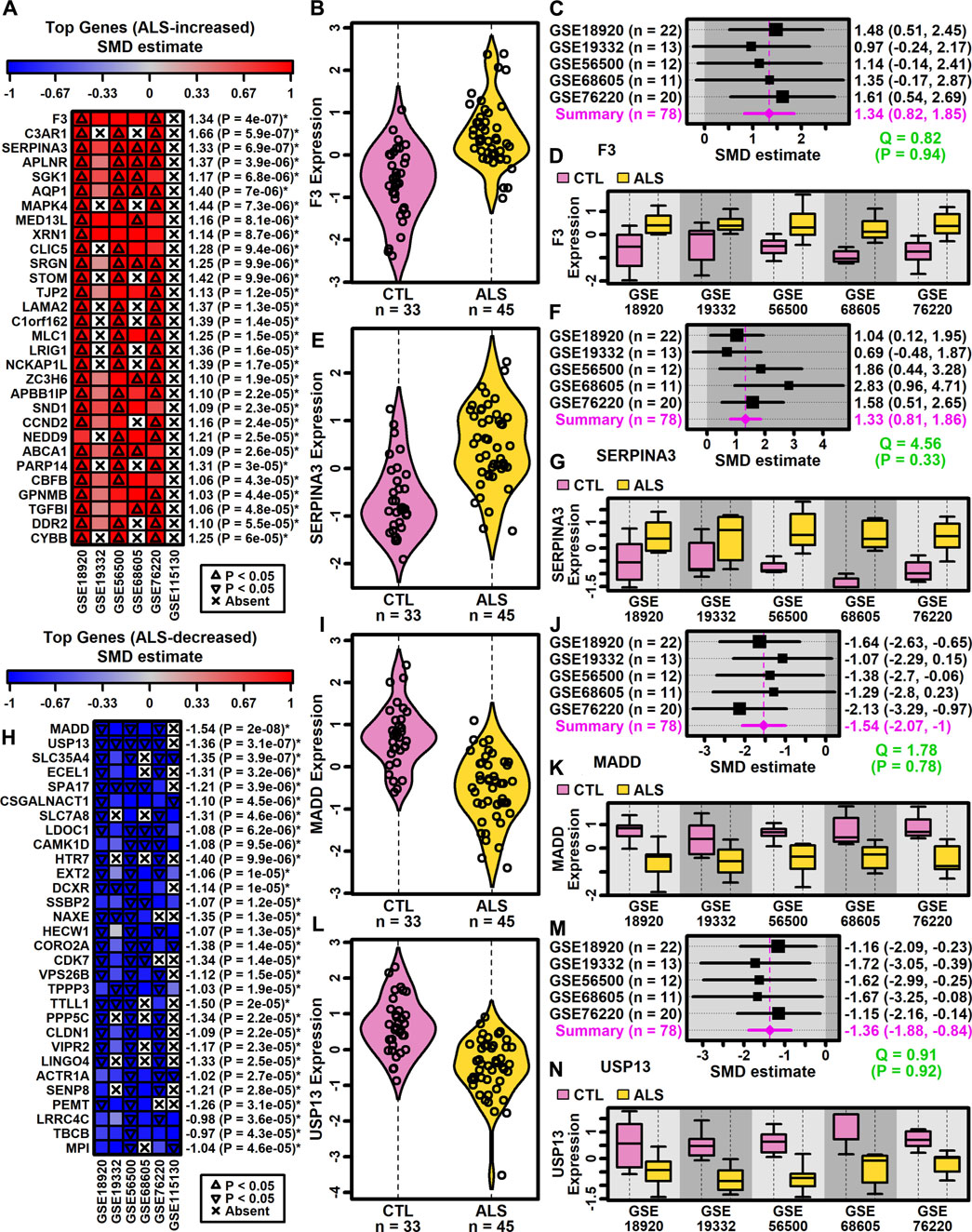
Figure 2. Top ranked meta-analysis genes. (A, H) Ranked list of (A) ALS-increased and (H) ALS-decreased genes. Heatmap colors reflect SMD estimates (see scale). The meta-SMD estimate is shown in the right margin with p-value (*FDR <0.10). (B, E, I, L) Violin plots. Log2-scaled expression values from each study were z-score normalized and combined. Gaussian kernal-based density estimates are plotted with expression values for each subject. (C, F, J, M) Forest plots. SMD point estimates are shown with 95% confidence intervals (right margin). The meta-SMD estimate is given in the bottom row (magenta font). Cochran’s Q test statistic for heterogeneity is shown with p-value (green font, bottom right). (D, G, K, N) Boxplots by study. Boxes outline the middle 50% of expression values for each group (whiskers: 10th to 90th percentiles). Log2-scaled expression values from each study were z-score normalized.

Genes most strongly decreased in ALS included MAP kinase activating death domain (MADD) and ubiquitin specific peptidase 13 (USP13) (Figures 2H–N). Both genes were ALS-decreased in the five datasets for which expression was detectably measured, with no significant effect size heterogeneity (Figures 2I–N). SMD for MADD ranged from −1.07 (GSE19332) to −2.13 (GSE76220) with an overall meta-estimate of −1.54 (p = 2 × 10−8; Figures 2H,J). Likewise, SMD for USP13 varied from −1.15 (GSE76220) to −1.72 (GSE19332) with an overall meta-estimate of −1.36 (p = 3.1 × 10−7; Figures 2H,M).

The 222 ALS-increased DEGs were most strongly associated with MeSH terms related to immunological processes, such as graft rejection, leukocyte chemotaxis, macrophage activation, cellular immunity and phagocytosis (Figure 3A; Supplementary Excel file S1). There were 390 Gene Ontology (GO) biological process (BP) terms enriched among the 222 ALS-increased DEGs (p < 0.05 with at least 2 ALS-increased DEGs per GO term), which could be organized into broad categories such as development, cell motility or taxis, signal transduction and response to external stimulus (Figure 3C). Specific GO BP terms most strongly enriched among ALS-increased DEGs included regulation of immune system process, blood vessel or circulatory system development and regulation of cell activation (Figure 3E). Gene set enrichment analysis (GSEA) confirmed that genes associated with regulation of immune system process were enriched among ALS-increased DEGs (p < 0.001; Figure 3G). The 222 ALS-increased genes were further enriched with respect to GO cell component (CC) terms, including plasma membrane, exosome, vesicle and cell periphery (Figure 3I). Other annotations most strongly enriched with respect to ALS-increased genes included extracellular matrix structural constituent (e.g., LAMA2, TGFBI, FN1), TYROBP causal network in microglia (e.g., NCKAP1L, APBB1IP, TYROBP), and spinal cord injury (e.g., AQP1, VCAN, AIF1) (Supplementary Excel file S1). Drug signature analysis showed that ALS-increased DEGs were enriched with genes targeted by dexamethasone, retinoic acid and the dopamine agonist pergolide (Supplementary Excel file S1).

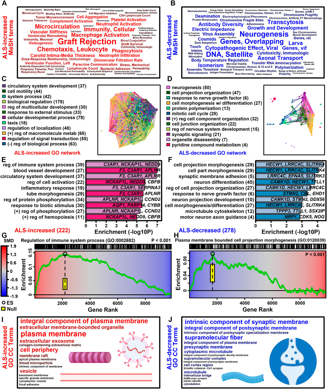
Figure 3. Functional enrichment analyses. (A and B) MeSH terms enriched among (A) ALS-increased and (B) ALS-decreased genes. MeSH term font size is inversely proportional to the enrichment p-value (Fisher’s Exact Test). MeSH terms were extracted from the gene2pubmed database (phenomena and processes category). (C and D) GO BP term network enriched among (C) ALS-increased and (D) ALS-decreased genes. Each node corresponds to a GO BP term with connections drawn between node pairs having ≥50% gene overlap. The complete set of enriched GO BP terms was clustered to form color-coded groups with the term having the largest number of genes listed as a representative. The number of GO BP terms within each group is given in parentheses. (E and F) Top-ranked GO BP terms. The most strongly enriched GO BP terms associated with (E) ALS-increased and (F) ALS-decreased genes are shown. Terms are ranked according to enrichment -log10-transformed p-values (horizontal axis). Representative genes are listed for each GO BP term and the total number of DEGs for each term is given in parentheses. (G and H) Gene set enrichment analysis (GSEA). Genes were ranked based upon SMD estimate (see color scale) and a running sum score was tabulated (green line) based on the position of genes linked to the indicated GO BP term (top margin). The enrichment score (black circle) is the running sum score with maximum absolute value. The yellow box outlines the middle 95% of the enrichment score null distribution from simulations in which the ranked gene list was randomly permuted (100000 trials). (I and J) Top ranked GO CC terms. All GO CC terms shown are significantly overrepresented among (I) ALS-increased DEGs (p < 0.001) or (J) ALS-decreased DEGs (p ≤ 0.019). The font size of each term is inversely proportional to its enrichment p-value.