LncRNAs are a class of non-coding RNAs transcribed from DNA with a length of over 200 nucleotides (Ponting et al., 2009). They account for 70%–80% of all non-coding RNAs and play crucial regulatory roles in numerous cellular processes, including but not limited to transcription, splicing, translation, DNA repair, and regulation of genes. The quantity and biological importance of lncRNAs determine their widespread involvement in all physiological activities of living cells and the pathogenesis of human diseases, such as cancer, Parkinson’s disease, and cardiovascular disease (Riva et al., 2016; Schmitz et al., 2016; McCabe and Rasmussen, 2021). LncRNAs represent a new type of potential therapeutic targets, that can affect the diagnosis, treatment, and prognosis of diseases, and have attracted significant attention (Blokhin et al., 2018; Fernandes et al., 2019; Winkle et al., 2021).

Due to the key roles of lncRNAs in diseases, it is crucial to develop lncRNA-targeted drugs and technologies. This presents a significant opportunity for the treatment of lncRNA-related diseases and represents a new area for drug development (Sangeeth et al., 2022). Emerging studies have shown that small-molecular drugs can inhibit the proliferation of tumor cells or tumor stem cells by regulating the expression of lncRNAs, laying a crucial theoretical foundation for the advancement of lncRNA-targeted therapeutics (Liu et al., 2021). To develop lncRNA-targeted drugs, it is necessary to take three preparatory steps: elucidating the action mechanism of lncRNAs in diseases, analyzing their structural and functional pockets, and finding small-molecular drugs that can bind specifically to the pockets. One important aspect of this process is identifying associations between lncRNAs and drugs (Jiang et al., 2019; Chen Y. et al., 2021). Predicting lncRNA-drug associations (LDAs) not only facilitates the selection of potential drug candidates but also streamlines the drug discovery process, ultimately propelling the realization of efficacious lncRNA-targeted therapies and fostering advancements in precision medicine.

LDAs are mainly identified through biological experiments. For example, curcumin plays a crucial role in the treatment of various cancers by regulating lncRNAs (Patel et al., 2020). It inhibits the expression of lncRNA H19, and restores MEG3 levels via demethylation, thus enhancing the sensitivity of cancer cells to chemotherapeutic drugs (Zhang et al., 2017; Cai et al., 2021). Wang et al. (2020) confirmed that the oncogenic factor lncRNA CCAT2 was overexpressed in ovarian cancer, and calcitriol, the vitamin metabolite, can inhibit the proliferation, migration, and differentiation of ovarian cancer cells by inhibiting the expression of CCAT2. However, identifying LDAs based on biological experiments is time-consuming and costly, there is a need for efficient and accurate computational methods to predict potential LDAs, which can be further verified by biological experiments.

Jiang et al. (2019) identified LDAs based on the hypothesis that lncRNAs with similar sequences are often regulated by the same drug, and drugs with similar structures tend to regulate the same lncRNA. Wang et al. (2018) utilized Elastic Network (EN) regression to predict potential LDAs by integrating lncRNA expression profiles and drug response data in cancer cells. However, the limitation of these methods is that they heavily rely on specific features of the existing data, which may affect the prediction performance. Although predicting LDAs is receiving increasing attention, the relevant prediction methods are still relatively lacking.

At present, a wealth of computational methods has been accumulated for predicting small molecule drug-miRNA associations (Qu et al., 2019; Yin et al., 2019; Chen et al., 2020). Considering that both lncRNAs and miRNAs are non-coding RNAs involved in gene expression regulation and cellular functions, and share similar regulatory mechanisms (Yan and Bu, 2021), the methods for predicting drug-miRNA interactions hold significant implications for predicting LDAs. Zhao et al. (2020) developed a model using symmetric nonnegative matrix factorization and Kronecker regularized least squares to predict small molecule drug-miRNA associations. Chen et al. (2021) predicted small molecule drug-miRNA associations based on bounded nuclear norm regularization. Wang et al. (2022) presented an ensemble of kernel ridge regression-based method to identify potential small molecule-miRNA associations. Niu et al. (2023) employed a combination of GNNs and Convolutional neural networks (CNNs) to predicted small molecule drug-miRNA association.

Recently, due to the breakthroughs in deep learning and the huge improvements in computing power, models based on deep learning, particularly those employing GNNs, have been applied in multiple bioinformatics-related tasks, such as lncRNA-disease association prediction, and drug-target interaction prediction (Xuan et al., 2019; Chen et al., 2020; Kumar Shukla et al., 2020; Zhao et al., 2023). Yin et al. (2023) proposed a general framework using residual GCN and CNNs to predict drug-target interactions. Wang and Zhong (2022) proposed a method (gGATLDA) to identify potential lncRNA-disease associations based on graph attention networks (GAT). The success of the above GNNs-based methods can be attributed to the three main reasons: 1) biological correlations can be modeled naturally as graph structures, 2) GNNs have the advantage of capturing complex network relationships, 3) the introduction of attention mechanisms enables the model to focus locally on important nodes in the graph and effectively integrate node information on a global scale.

Therefore, based on the experiments validated LDAs dataset (D-lnc (Jiang et al., 2019)), we propose a GNNs-based framework to predict LDAs by referring to the gGATLDA method which was originally designed to predict lncRNA-disease associations. In this paper, we first extract the lncRNA-drug bipartite graph according to the LDAs matrix and obtain one-hop enclosing subgraphs of all lncRNA-drug pairs from the bipartite graph. Then, the feature vectors of lncRNA-pairs are constructed according to Gaussian interaction profile kernel lncRNA (drug) similarities. Finally, GCN learns lncRNA and drug node embeddings and obtain local spatial characteristics of nodes. GAT uses the attention mechanism to integrate the global information of the lncRNA-drug bipartite graph. Our model takes full advantage of GCN and GAT to predict novel LDAs. Results show that the method achieves high AUC and AUPR, and the ablation experiments show that our model performs better than GCN and GAT. The case studies on two drugs (Berberine and Panobinostat) and two lncRNAs (NEAT1 and MEG3) demonstrate the effectiveness of the model in predicting the potential LDAs. In the functional enrichment analysis, we further verified the validity of our predicted LDAs from the perspective of the relationship between the biological function of drugs and the enrichment pathway of lncRNA target genes. All these results suggest that the framework used in this study is an efficient method for predicting LDAs.

Three benchmark datasets including the Gene Expression Omnibus (GEO) dataset, Connectivity Map (cMap) dataset, and Validated dataset (Jiang et al., 2019) are downloaded from http://www.jianglab.cn/D-lnc/index.jsp. The cMap dataset and GEO dataset were obtained by re-annotating microarray probes in cMap and GEO databases, respectively, and screening lncRNA differential expression data before and after drug therapy. The Validated dataset was created by searching experimentally verified drug modification of lncRNA expressions. We obtain three benchmark datasets (Dataset 1, Dataset 2, and Dataset 3) by removing the repeated LDAs of GEO dataset, cMap dataset, and Validated dataset respectively. As the number of lncRANs and drugs in three benchmark datasets is unbalanced, only when Dataset 1 and Dataset 2 are combined, the number of them is relatively balanced. Therefore, we combine Dataset 1 and Dataset 2 into Dataset 4, which is used as a training dataset in the case study to predict LDAs in Dataset 3 (see case study section). Dataset 5 is merged from Dataset 1, Dataset 2, and Dataset 3. Table 1 shows the detailed information of five datasets. We treat the known LDAs as positive samples and randomly select the negative samples with the same number of positive samples from the unknown LDAs.

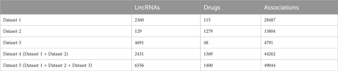
Table 1. The detailed information of five datasets.

The flowchart of the method is shown in Figure 1. Firstly, construct the lncRNA-drug association matrix, lncRNA similarity matrix, and drug similarity matrix. Secondly, construct one-hop enclosing subgraphs according to the lncRNA-drug bipartite graph, and obtain lncRNA node features and drug node features, respectively. Further, the one-hop enclosing subgraph of each lncRNA-drug pair and their feature vectors are input to the GNNs model. Finally, the lncRNA vector and drug vector are concatenated and processed by Softmax to obtain the prediction score.

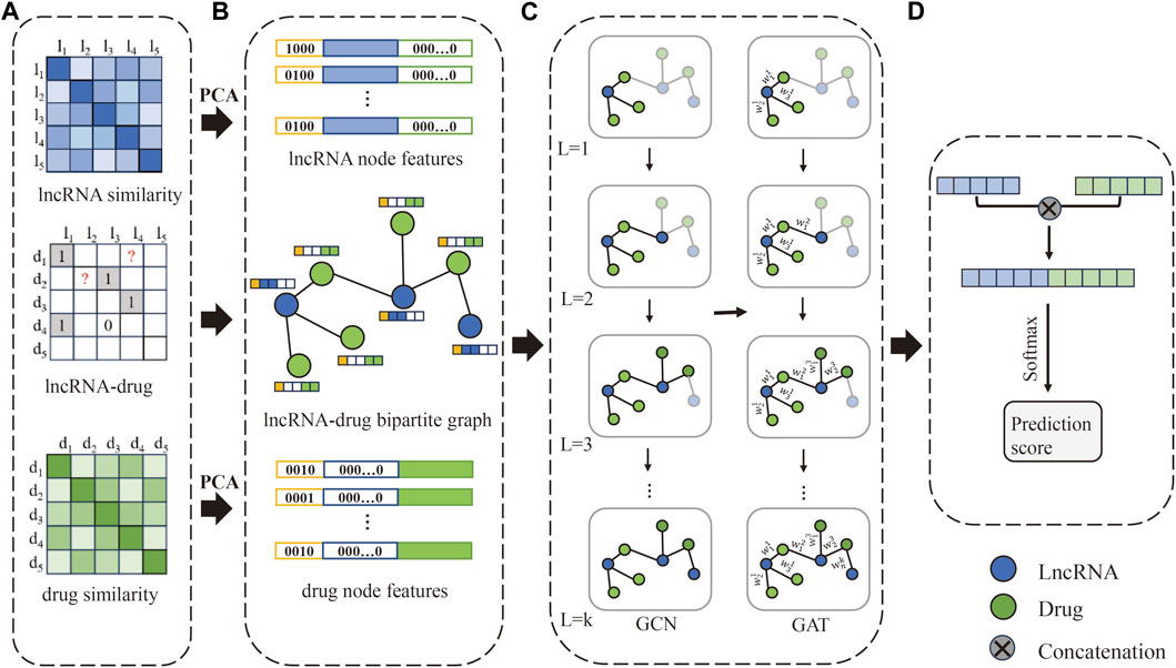
Figure 1. The flowchart of our method. (A) The LDAs matrix, lncRNA similarity matrix, and drug similarity matrix are constructed, respectively. (B) Obtain lncRNA-drug bipartite graph and one-hop subgraphs, and construct the initial feature vector of lncRNA and drug. (C) Extract feature representation of lncRNAs and drugs based on GCN and GAT. (D) Concatenate the lncRNA vector and drug vector to obtain a new vector, and the prediction score is obtained by Softmax.

Because of the sparsity of the lncRNA-drug association matrix LD∈Rm×n, we calculate lncRNA similarity LSli,lj and drug similarity DSdi,dj by the following Gaussian interaction profile kernel (GIP) (van Laarhoven et al., 2011; Yang and Li, 2021):

where LS∈Rm×m and DS∈Rn×n denote the lncRNA similarity matrix and drug similarity matrix, respectively. m and n represent the number of lncRNAs and drugs respectively. IPli and IPdi are binary vectors, which represent the i th row and i th column of LD, respectively. If lncRNA li is associated with drug dj, LDi,j=1, otherwise LDi,j=0. rl and rd are used to adjust the kernel bandwidth, which are calculated as followed:

The bipartite graph G is constructed from the matrix LD, where each known lncRNA-drug pair corresponds to an edge connecting the lncRNA li and drug dj, for unknown LDAs, there are no edges between li and dj. The one-hop enclosing subgraph G1V1,E1 of each lncRNA-drug pair li,dj can be defined as following: V1 is the set of nodes containing one-hop neighbor nodes of li, one-hop neighbor nodes of dj, as well as node li and node dj, and E1 is edge set. Each node in subgraphs can be labeled to distinguish its role (Zhang and Chen, 2020). We use 0 and 1 to label target lncRNA node and target drug node, respectively, and use 2i and 2i+1 to label the one-hop neighbor nodes of li and the one-hop neighbor nodes of dj, respectively, where i represents the order of neighbor nodes, and it is set to 1 according to gGATLDA (Wang and Zhong, 2022).

We initially explore the influence of various hyperparameter combinations on the performance of predicting LDAs across five datasets. These hyperparameters include epochs, batch size, learning rate, the initial feature vector dimensionality selected by PCA, and the layers of GCN and GAT, respectively. We utilize grid search to tune these six hyperparameters. The epochs range extends from 10 to 50, incremented by 10. Batch size is selected from the set , learning rate is chosen from , and the initial feature vector dimensionality selected by PCA ranges from . The experimental results are shown in Figure 2, the optimal model performance is attained when a particular combination of hyperparameters is used on Dataset 1 to Dataset 5. Specifically, epochs are set to , batch sizes to , and learning rate uniformly to 0.001. Additionally, the number of initial PCA-selected feature dimensions is set to for each dataset.

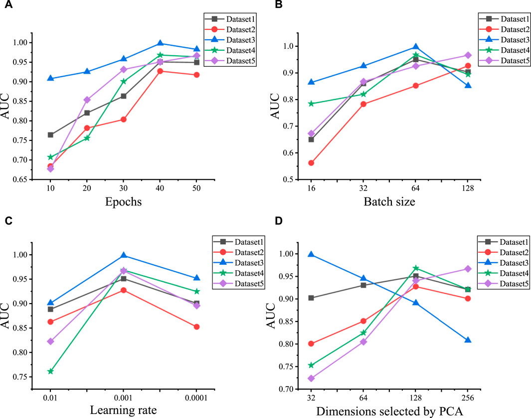
Figure 2. Hyperparameter optimization results for five datasets. (A) The AUC values under the different epochs on five datasets. (B) The AUC values under the different batch sizes on five datasets. (C) The AUC values under the different learning rates on five datasets. (D) The AUC values under the different dimensions selected by PCA on five datasets.

In addition, the selection of model structure is crucial for prediction performance. Therefore, we also investigate the impact of the two main hyperparameters, the number of GCN and GAT layers on the model in Dataset 1, Dataset 2, and Dataset 3. Specifically, we select layer numbers ranging from 1 to 3 for both GCN and GAT. The increase in the number of GNN layers means aggregating features from higher-order neighbor nodes, but it may lead to the loss of local structure, resulting in overfitting and decreased prediction performance. For instance, as shown in Table 2, in Dataset 1, increasing the GCN layer from 1 to 2 improves performance, but further increasing it to 3 leads to a decrease in performance. It is worth noting that the model achieves the best performance across all three datasets when the model structure consists of 1 GCN layer and 3 GAT layers. Therefore, we choose 1 GCN layer and 3 GAT layers as our model architecture.

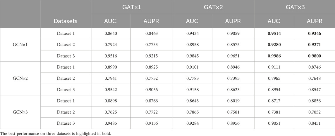
Table 2. The performance using different numbers of GCN and GAT layers on Dataset 1, Dataset 2, and Dataset 3.

To avoid potential random bias, we repeat the five-cross-validation process 100 times and average the performance metrics to derive the final results. The results are shown in Table 3, the AUC and AUPR are higher than 0.92 on both the benchmark datasets and combined datasets. It is noteworthy that the overall performance of the model is superior on the combined datasets compared to the benchmark datasets. For instance, among the benchmark datasets, the model on Dataset 1 and Dataset 2 achieves the AUC of 0.9514 and 0.9280, respectively. However, the model’s AUC on Dataset 4 (Dataset 1+Dataset 2) is 0.9690, which surpassed that of its constituent subsets. This improvement of performance on the combined dataset can be attributed to the more balanced relationship between the quantities of lncRNAs and drugs and the more trainable data in this dataset. However, on the contrary, the performance of benchmark Dataset 3 is better than that of the combined datasets. This discrepancy can be attributed to the presence of 4791 LDAs involving 4691 lncRNAs and 48 drugs in Dataset 3. Notably, the average degree size of each drug is 99, implying that one drug corresponds to multiple lncRNA information, enabling the model to extract more complex features from abundant lncRNA information. Consequently, it facilitates a more accurate capture of the relationship between drugs and lncRNAs. Overall, these observations indicate that the proposed method has an excellent performance on the five datasets.

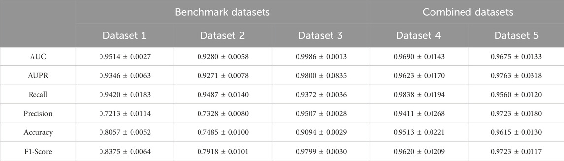
Table 3. The performance of the method on five datasets.

To further study the influence of GCN and GAT on the model performance, we also conduct ablation experiments on five datasets. Specifically, we individually use the GCN and GAT modules, as well as their combined module for LDA prediction. As shown in Figure 3, among the three modules, the combined GCN and GAT modules obtain the optimal performance across all five datasets, followed by the GAT module, with the GCN module exhibiting the poorest performance. GCN module learns the feature representation of lncRNA and drug nodes by aggregating their neighbor information, which enables GCN to capture the spatial local structure of nodes. GAT module introduces an attention mechanism that allows the model to dynamically assign weights and integrate the global information of the lncRNA-drug bipartite graph, rather than just the neighbors of the lncRNA and drug nodes. Therefore, combining GCN and GAT modules enables the model to take full advantage of their strengths, complement each other, and further improve the prediction performance.

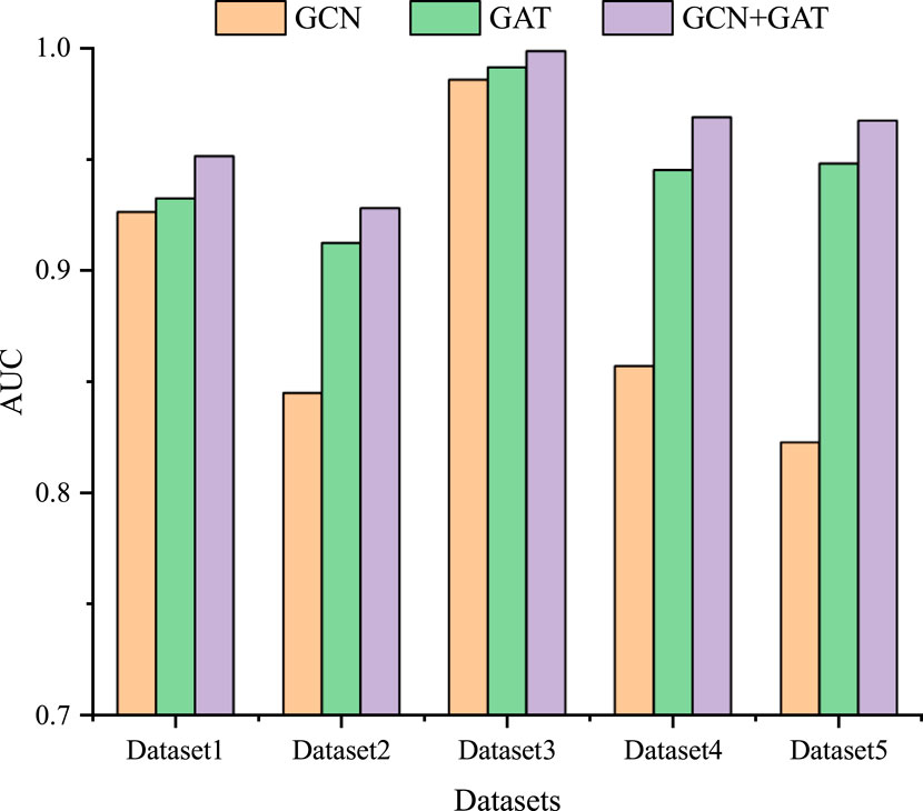
Figure 3. The results of the ablation experiment on five datasets.

Figure 4 shows the top 10 predicted LDAs for the two drugs and two lncRNAs where the line width indicates the magnitude of the association score and the green lines indicate the confirmed LDAs in the test datasets. The blue lines indicate those LDAs that are not confirmed by the test dataset but have literature support. Generally, all the confirmed associations have large predicted scores. The red dotted lines represent LDAs having no support indication up to now. As shown in Figure 4A, 8 out of 10 predicted lncRNA-Berberine associations are validated, among which lncRNA “MALAT1” and “H19” are confirmed in the literature. Cao et al. (2020) demonstrated that lncRNA MALAT1 in cerebral ischemia was significantly reduced after treatment with the drug Berberine, highlighting its anti-inflammatory effects in mice after MCAO surgery. Song et al. (2022) identified lncRNA H19 as a potential key regulatory lncRNA of Berberine. Among the top 10 lncRNAs predicted associated with Panobinostat (Figure 4B), 8 lncRNAs are confirmed in test datasets. And for lncRNA NEAT1, 6 out of 10 predicted drugs related to NEAT1 are verified (Figure 4C). And 8 predicted drug-MEG3 associations have evidence in test datasets and literature (Figure 4D).

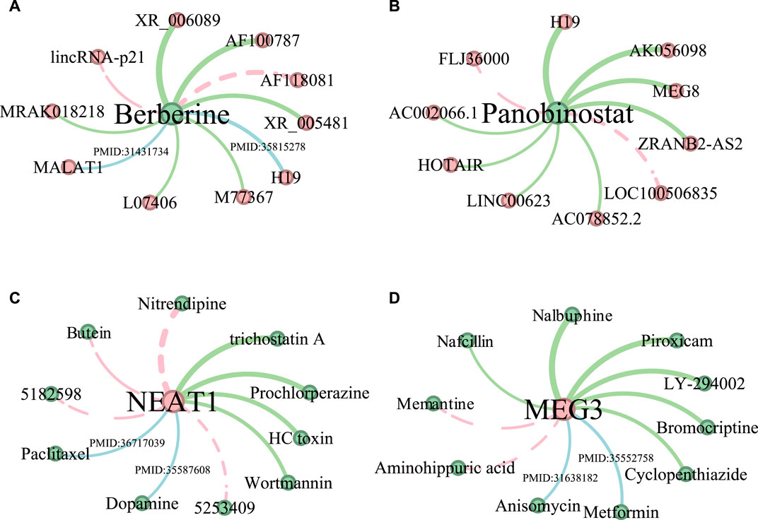
Figure 4. The predictive results of the top 10 lncRNAs associated with drugs Berberine (A) and Panobinostat (B), and the top 10 drugs related to lncRNA NEAT1 (C) and MEG3 (D). LncRNAs are represented by red nodes, while drugs are denoted as green nodes. The thickness of the edge indicates the predicted ranking, and the thicker the edge, the higher the ranking. Moreover, the LDAs found in test datasets are shown in green edges. Associations supported by existing literature are shown in blue edges, accompanied by their corresponding PMID references. Unconfirmed associations are represented by red dotted edges.

Since one lncRNA may regulate the expression of multiple downstream genes, therefore intervening with one lncRNA may involve a variety of biological functions. In addition, a drug may target a certain lncRNA to alter its expression, thereby regulating the expression of lncRNA target genes or modifying the activity of signaling pathways to realize its biological functions. For instance, Guo et al. (2016) showed that aspirin could significantly induce the expression of lncRNA OLA1P2 in human colorectal cancer, thereby affecting the activity of the STAT3 signaling pathway. To gain insights into the functional implications of the drugs and lncRNAs of concern, we conduct functional enrichment analysis on their related genes by an online tool DAVID (Sherman et al., 2022), which is widely used for functional annotation and enrichment analysis of gene lists.

Based on the results of the first part of the case study, firstly, we perform functional enrichment analysis on the target genes of lncRNAs predicted associated with two drugs (Berberine and Panobinostat). We search the literature demonstrating that drug functions are related to the enrichment pathways of lncRNA target genes. In Figure 5A, among the top 15 KEGG pathways of Berberine-related lncRNA target genes, 12 have been confirmed associated with the existing functions of Berberine. For example, Ayati et al. (2017) demonstrated that Berberine can play an anticancer role by regulating the expression of oncomiRs and tumor-suppressive miRs in various cancer cells (Hepatocellular carcinoma, gastric cancer, ovarian cancer, colorectal cancer). Okuno et al. (2022) evidenced that Berberine overcomes gemcitabine-related chemical resistance by modulating rap1/PI3K-akt signaling in pancreatic ductal adenocarcinoma. In Figure 5B, there are 12 KEGG pathways of predicted Panobinostat-related lncRNA target genes that are found to be associated with the functions of Panobinostat. Lee et al. (2017) demonstrated that Panobinostat overcame resistance to gefitinib in KRAS-mutant/EGFR wild-type non-small-cell lung cancer by targeting TAZ. Studies have also shown that Panobinostat can restore the sensitivity of endocrine-resistant and triple-negative breast cancer cell lines to estrogen receptors (Tan et al., 2016).

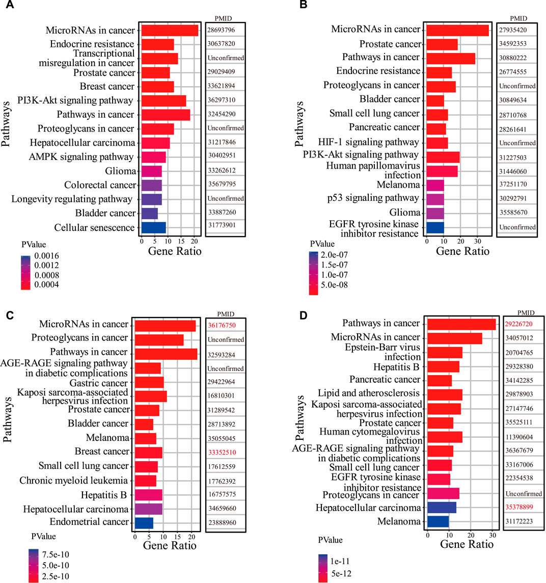
Figure 5. The results of functio