The human microbiome consists of trillions of microbes that reside inside and outside the human body, and these microbes play an essential role in maintaining the overall health of the human body (Ogunrinola et al., 2020). The host-microbe plays a crucial role in several physiological processes in the human body, such as energy collection and storage (Amato et al., 2019), facilitating carbohydrate absorption, and protecting the body from foreign microorganisms and pathogens (Hajiagha et al., 2022). Moreover, the changes in microbiota composition can significantly affect human health Kim et al. (2018); Partula et al. (2019); Catinean et al. (2018). Many studies have shown that the dysbiosis or unbalance of microbiota is closely related to disease, and the microbiota is an important causative factor for many diseases. Therefore, microbes are considered new therapeutic targets for precision medicine (Cullin et al., 2021), and the research on the relationship between microbes and drugs not only aids in drug development but also the diagnosis and treatment of human diseases. However, the popularization and widespread use of antibiotics in modern medicine have led to the emergence of an increasing number of drug-resistant microbes, which seriously threaten human health (Pugazhendhi et al., 2020). Although many researchers have provided extensive evidence on the association between microbes and drugs, traditional biomedical experiments are time-consuming, labor-intensive, and costly (Paul et al., 2010). These reasons hinder the efficiency of drug development and hardly satisfy the massive demands for novel drugs. Therefore, it is necessary to explore the microbe-drug associations at a large-scale level for drug development.

To overcome the above challenges, computational models have emerged as an effective method for identifying microbe-drug associations, and these models are used to predict microbe-drug associations by integrating different genomic information, including genomics, macro genomics, and metabolomics. With the rapid development of high-throughput sequencing technology and advanced genomics techniques, the research on microbe-drug association prediction has developed rapidly, generating a large amount of valuable research data. To further investigate the potential association between microbes and drugs, a series of microbe-drug association databases have been constructed in recent years, such as aBiofilm (Rajput et al., 2018), MDAD (Sun et al., 2018) and DrugVirus (Andersen et al., 2020), which have immensely promoted the development of microbe-drug association prediction models. Over the past few years, many computational models have emerged that utilize the above databases to infer potential associations between microbes and drugs. As an illustration, Zhu et al. proposed a computational method, HMDAKATZ, which applied the KATZ measure to predict inherent associations between microbes and drugs (Zhu et al., 2019b). Long et al. (2020) proposed a computational method called GCNMDA, which combined graph convolutional networks (GCNs) and conditional random fields (CRFs) with an attentional mechanism aiming to identify the hidden associations between microbes and drugs. In 2021, GATMDA was proposed, which utilized inductive matrix completion and graph attention networks (GNNs) to predict associations between microbes and diseases (Long et al., 2021). The Graph2MDA model combined the constructed multimodal attribute graphs and variational graph autoencoder (VGAE) to predict microbe-drug associations accurately (Deng et al., 2022). GSAMDA is likewise a microbe-drug association prediction model, which primarily applies graph attention networks (GATs) and sparse autoencoders (Tan et al., 2022). The computational model NIRBMMDA (Cheng et al., 2022) combines neighborhood-based inference (NI) and restricted Boltzmann machine (RBM) methodologies to predict Microbe-Drug Associations (MDA). By leveraging NI, it extracts proximity information from microbes or drugs, while RBM is used to learn the latent probability distribution inherent in the known association data. This integrative approach harnesses the strengths of both components, resulting in a more robust predictive framework. In the study of Tian et al. (2023), they proposed the SCSMDA model, which was based on GCN and integrated structure-enhanced contrast learning and self-paced negative sampling strategies to improve the accuracy in microbe-drug association prediction. In addition, the GACNNMDA model integrated a GTA-based autoencoder and a CNN-based classifier, which transforms multiple attribute combinations of the microbes and drugs into two feature matrices to predict the associations of the microbes and drugs (Ma et al., 2023). Qu et al. (2023) proposed MHBVDA to predicts virus-drug associations by integrating multiple biological data sources and employing integrating two matrix decomposition-based methods. And it innovatively applies Bounded Nuclear Norm Regularization (BNNR) with regularization terms to mitigate the impact of noisy data and overfitting issues, thereby enhancing prediction accuracy. However, these methods based on graph neural networks still have room for improvement in prediction performance. When multi-layer networks are stacked, there is some confusion between different orders of neighborhood information, the node representations become indistinguishable, and the network performance decreases, which tends to prevent GNN with multiple layers from effectively utilizing the higher-order neighborhood information (Li et al., 2018).

Therefore, to achieve better prediction performance, inspired by the work of Song et al. (2023), this paper proposed an ordered gating mechanism-based ordered message-passing GNN method to infer potential microbe-drug associations, called OGNNMDA. In OGNNMDA, the known association data are preprocessed to compute Gaussian interaction profile kernel similarity and additional biomedical information similarity (microbe functional similarity, drug structural similarity) for drugs and microbes, respectively. Then, the multiple similarity matrices are fused and stitched together to obtain the heterogeneous networks. The heterogeneous network was fed into the encoder consisting of the two-layer fully connected network and the 12-layer ordered message-passing GNN to derive embedding representations of the drugs and microbes, respectively. Finally, the bilinear decoder was adopted to reconstruct the microbe-drug association matrix to infer possible associations between the microbes and drugs. Furthermore, to evaluate the predictive performance of OGNNMDA, in-depth comparative experiments, ablation experiments, and case studies are conducted in this paper. The results demonstrate that OGNNMDA outperforms current representative existing methods and achieves satisfactory results in potential drug-microbe association prediction.

All the aBiofilm, MDAD and DrugVirus datasets provide important insights into the complex interactions between the drugs and the microbes, providing researchers in the fields of bioinformatics and graphical neural networks with a wealth of information to analyze and utilize to advance their studies and methods. The basic statistical information of the three datasets is presented in Table 1.

In 2018, Rajput et al. introduced the aBiofilm (http://bioinfo.imtech.res.in/manojk/abiofilm/) dataset, which is of great significance for the development of the bioinformatics and graph neural network fields (Rajput et al., 2018). Over the last three decades, many anti-biofilm agents have been experimentally verified to disrupt biofilms. aBiofilm organizes these data, which contain a database, a predictor, and a data visualization module. The database contains biological, chemical, and structural details of 5,027 anti-biofilm agents (1720 different ones) reported from 1988 to 2017. After eliminating redundant associations among them, a total of 2,884 known interaction associations of 1720 drugs and 140 microbes were finally obtained.

MDAD (https://github.com/Sun-Yazhou/MDAD/) is also a valuable microbe-drug association dataset, which was proposed by Sun et al. based on a variety of drug-related databases as well as a large amount of literature (Sun et al., 2018). Specifically, MDAD contains 5,505 associations between 180 microbes and 1,388 drugs collected from 993 documentation. After filtering out redundant information, a total of 2,470 microbe-drug associations were obtained, involving 173 microbes and 1,373 drugs.

DrugVirus (https://drugvirus.info/) compiles interactions involving 118 virus-targeting drugs and 83 human viruses, encompassing SARS-CoV-2 (2019-nCoV) (Andersen et al., 2020). Building upon this foundation, Lond et al. systematically extracted and curated 57 drug-virus associations from pertinent drug databases and scholarly publications, which involved 76 unique drugs and 12 distinct viruses. Ultimately, they assembled a dataset comprising 175 drugs and 95 viruses, yielding a total of 933 documented drug-virus interaction records.

In this section, firstly, the definition of the association adjacency matrix is given, secondly, the similarity calculation of drugs and microbe based on the adjacency matrix is given, and finally, the heterogeneous network is obtained based on multiple similarities.

For simplicity, for each dataset, let D=d1,d2,…,dNd denote the set of different drugs, and M=m1,m2,…,mNm denote the set of different microbes. Therefore, a primitive known microbe-drug association network Net=D∪M,E can be constructed: for each given drug di1≤i≤Nd and microbe mj1≤j≤Nm there exists a unique edge corresponding to it in E if and only if there is a known association between them. Based on the above definition, the adjacency matrix A∈RNd×Nm can be obtained as shown in Eq. 1.

Ai,j=1…Lconv, hvl∈R1×k is the embedding feature of the layer l, Nv denotes the set of neighboring nodes for the node v, Lconv corresponds to the number of layers in the GNN network and the number of message-passing rounds. The dimension of the node’s embedding feature is denoted by k. In this study, the final embedding dimension is set to match the embedding dimensions used across the GNN layers. H is the microbe-drug heterogeneous network graph defined in Eq. 8, which is processed for embedding and provides edge information for the GNN. The node representation h0∈RNd+Nm×k is obtained by a two-layer MLP defined by Eq. 10 and 11. The trainable variables Wfc1,Wfc2∈RNd+Nm×k and Bfc1,Bfc2∈Rk are involved in this process. Additionally, Hinit∈RNd+Nm×Nd+Nm represents the initial node representation, and σ denotes the ReLU activation function.h0=σWfc2σWfc1Hinit+Bfc1+Bfc2(10)

The function ϕ calculates the messages transmitted between nodes, where the edge attribute is directly used as the message. The symbol □ represents the message aggregation function, and in this paper, the mean method is employed (Huan et al., 2021). This means that messages received from multiple neighboring nodes are aggregated by taking their average, resulting in message characteristics used for updating node representations. Finally, γ represents the node representation update function, which implements the ordered message-passing mechanism discussed in this paper.

In the message-passing process of a single-level GNN, a node only exchanges messages with its immediate neighbors. This pattern of neighbor message transmission at different orders aligns with the structure of the node root tree in a multi-layer GNN (Liu et al., 2020). As illustrated in Figure 2, for a node v, Nvl represents the neighbor information of node v at the lth layer, and the nesting relationship of its neighbor messages at each layer can be described using Eq. 12.

Nv1⊆Nv2⊆⋯⊆NvLconv(12)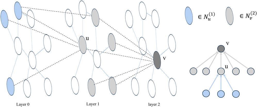

Figure 2. Taking a two-layer GNN as an example, layer 0 represents the initial node embedding, and the adjacency of nodes between layers forms multiple trees. In the figure, u is a neighbor node of v. Nv(2) and Nu(1) are shown in the image with two colors respectively. The right side shows the tree structure of neighbor information with v node as the viewpoint, and the arrow represents the direction of neighbor information transfer.

In single-layer message passing, direct-neighbor node messages and higher-order neighbor node messages are differentially encoded to ensure orderly message delivery. Specifically, the neuron rows are aligned with the node root tree at each layer, enabling the acquisition of node feature representations with consistent nesting relationships. To implement this alignment encoding method, the neurons can be ordered by linearly arranging the neurons of each layer and considering a segmentation point, denoted as s. The information of the neighbors of the current node v, at order one or higher, can be encoded as svl (Song et al., 2023). The segmentation point s corresponds to the nested nature of node v, and its size relationship is determined by Eq. 13.

sv1≤sv2≤⋯≤svLconv(13)

Next, we describe the node feature update function γ, which is exemplified below for a specific node v. The function can be divided into three distinct steps.

1. Compute the aggregated message representation ml∈RNd+Nm×k for layer l.

2. For node v, this paper utilizes the gating vector ĝvl of dimension Nd+Nm to describe the segmentation point svl. Specifically, the value of the left part 0,svl−1 is set to 1, indicating the neighboring neurons of node v that are higher than the first order. Conversely, the value of the right part svl,Nd+Nm−1 is set to 0, denoting direct neighboring neurons. This is achieved by calculating the cumulative sum of the probability that each position in the node servers as a split point svl. The expectation gating vector ĝvl is obtained through a biased linear projection of the node representation vector in layer l − 1 and the message vector in layer l, as shown in Eq. 15.

ĝvl=cumsum←softmaxhvl−1;mvlWgl+Bgl(15)

In Eq. 15, the trainable parameters Wgl∈R2k×k and Bgl∈Rk are utilized. Additionally, hvl−1;mvl represents the concatenation of two vectors hvl−1 and mvl. To ensure that the predicted gated vector ĝvl adheres to the relative size relationship of the splitting points mentioned earlier, the operation described in Eq. 16. This operation yields the final gated vector gvl.

gvl=gvl−1+1−gvl−1⋅ĝvl(16)

3. Equation 17 demonstrates the utilization of the gating vector gvl to regulate the integration of the layer l − 1 node representation hvl−1 with the layer l aggregated context mvl. This process results in the acquisition of the new node representation hvl.

hvl=LNgvl⋅hvl−1+1−gvl⋅mvl(17)

In Eq. 17, the symbol ⋅ represents element-by-element multiplication, and LN refers to the layer normalization operation (Chen et al., 2022).

4.2 Decoder

After the previous rounds of the ordered message passing process, the final node embedding representation hLconv∈RNd+Nm×k is obtained. This representation can be considered as the concatenation of the final embedding features of the drugs, hd∈RNd×k, and the microbes, hm∈RNm×k. In this paper, the final embedding features hd and hm are obtained separately using the matrix splicing approach defined in Eq. 18.

To reconstruct the adjacency matrix A′ representing possible microbe-disease associations, the bilinear decoder is employed. It is a structural component employed for predicting the probability of potential edges or links based on node embedding vectors. These decoders commonly integrate the embedding vectors of node pairs within a graph to generate a score function that assesses the likelihood of a link between two nodes. The key characteristic of bilinear decoders lies in their utilization of bilinear transformations to capture the interaction effects among nodes. Specifically, for a drug node and microbe node pair (u, v) with their respective embedding vectors hd(u) and hm(v), a bilinear decoder might compute the score by Eq. 19.

scorehdu,hmv=hduTWhmv(19)

Where W is a learnable weight matrix. This score can be interpreted as the probability of link occurrence after a nonlinear activation function transformation, so that A′ can be obtained by the bilinear decoder as shown in Eq. 20.

In the above formula, where WB∈Rk×k represents a trainable matrix and σx=1/1+e−x is the sigmoid function. Overall, the complete computational flow of OGNNMDA can be seen in Algorithm 1.

Algorithm 1.OGNNMDA.

Require: Known associations matrix A∈RNd×Nm, drug similarity matrix DS∈RNd×Nd, microbe similarity matrix MS∈RNm×Nm and α = 600 is the number of iterations for OGNNMDA

Ensure: The constructed drug-microbe associations matrix A′∈RNd×Nm

  1:  Construct the heterogeneous network H according to formula (8)

  2:  Initialize the embedding feature matrix Hinit according to formula (11).

  3:  Initialize the gate vector = 0

  4:  for i = 1 → α do

  5:   calculate h0 according to formula (10)

  6:   for l = 1 → Lconvdo

  7:    calculate message matrix ml formula (14).

  8:    calculate ĝl by formula (15)

  9:    calculate g̃l formula (16)

  10:    calculate hl formula (17)

  11:   end for

  12:   get the embedding feature for drugs and microbes with hd and hm according to formula (18)

  13:   get the reconstruction matrix A′ by formula (20)

  14:  end for

4.3 Optimization

During the experiment, positive samples were the drug-microbe pairs with known associations, while negative samples were the drug-microbe pairs without known associations. These sets of positive and negative samples are denoted as Ω+ and Ω−, respectively, for ease of description. It is important to note that the number of pairs with known associations in both the aBiofilm dataset and the MDAD dataset is significantly smaller than the number of pairs without known associations. Therefore, when training OGNNMDA, the loss function incorporates a weighted cross-entropy loss, as defined in Eq. 21.

L=−1Nd×Nmλ∑i,j∈Ω+logai,j′+∑i,j∈Ω−log1−ai,j′(21)

In the above formula, (i, j) represents a pair of the drug di and microbe mj. λ is introduced as a balancing factor, calculated as the ratio of the number of samples in Ω− to the number of samples in Ω+. This factor helps attenuate the impact of data imbalance and emphasizes the reinforcement of known correlation information.

In this paper, the Xavier initialization method (Duong et al., 2019) is employed to initialize the trainable parameter matrices in various components of the model. These include the 2-layer fully connected layer, the ordered message-passing graph neural network layer, the bilinear decoder, and others, denoted as Wfcl,Bfcl|Wfcl∈RNd+Nm×k,Bfcl∈Rk,1≤l≤Kfc, Wgl,Bgl|Wgl∈R2*k×cs,Bgl∈Rcs,1≤l≤Kconv, and the bias matrix WB∈Rk×k. Furthermore, the Adam optimizer (Wang et al., 2023) is utilized to minimize the loss function. Adam combines the benefits of momentum optimization and adaptive learning rate, enabling quick convergence and adaptation to different parameter learning rates during the training process. This optimization technique enhances the training effectiveness of the deep learning model.

To prevent overfitting, the paper introduces node dropout (Piotrowski et al., 2020) and regularized dropout (Berg et al., 2017) schemes in the graph convolution layer. Node dropout can be seen as training multiple models on various sub-nodes, and the combination of these sub-nodes is used to predict unknown microbe-drug pairs (Tan et al., 2020).

5 Results

This paper begins by providing a brief overview of the experimental setup and the analysis and selection of certain hyperparameters. The aim is to validate the predictive performance advantages of OGNNMDA through intensive comparison experiments. These experiments involve 6 representative microbe-drug association prediction models, including state-of-the-art approaches. The evaluation is conducted on three well-known public datasets, namely, aBiofilm, MDAD and DrugVirus, within a 5-fold cross-validation framework. Furthermore, ablation experiments are performed to investigate the effectiveness of the ordered message-passing mechanism employed in OGNNMDA. Finally, a case study is presented to validate OGNNMDA using two commonly used drugs, ciprofloxacin and moxifloxacin, along with two common oral microbes, Actinobacillus aggregatum and Clostridium nucleatum.

5.1 Experimental parameter setting

In this paper, all experimental evaluations are conducted within a five-fold cross-validation setup. To ensure statistical robustness, each method is executed ten independent times for every experiment, thereby enabling the calculation of the mean value for each performance metric across these repetitions. In detail, this involves dividing all known associations in the dataset equally into 5 parts, denoted as testp=tp1,tp2,tp3,tp4,tp5. Additionally, a subset of the same size as the known associations is randomly selected from the unknown association set. This subset is divided equally into 5 parts, denoted as testn=tn1,tn2,tn3,tn4,tn5.

During the i − th (1 ≤ i ≤ 5) cross-validation iteration, the training set is defined as traini=testp−tpi, and the test set is defined as testi=tpi∪tni. The final test result of the 5-fold cross-validation experiment is calculated based on the combined test set, test = testp ∪ testn.

Based on the previous description of the model structure, OGNNMDA incorporates several hyperparameters, including the dimension size (k) of embedded features, the number of fully-connected layers (Lfc), the number of ordered message-passing GNN layers (Lconv), the initial learning rate (r) of Adam’s optimizer, the total training period (α), the node dropout metrics (β), and the regularized dropout parameter (γ).

To establish initial values for these parameters, we set Lfc = 2, r = 0.008, α = 600, β = 0.6, and γ = 0.4. Subsequently, we examine the effects of different values for parameters k and Lconv through experimental analysis.

To investigate the impact of different hyperparameter values on the model, this paper performed 5-fold cross-validation (5 cv) experiments on the aBiofilm and MDAD datasets. The results for the AUROC were plotted in Figure 3, showcasing the outcomes for various combinations of the parameters Lconv and k.

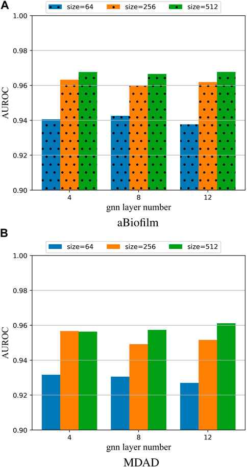
Figure 3. (A) Model hyperparameter analysis on the aBiofilm dataset. (B) Model hyperparameter analysis on the MDAD dataset.

From Figures 3A, B, it is evident that the optimal combination of Lconv and k is Lconv = 12 and k = 512. Therefore, this parameter setting will be utilized for OGNNMDA in subsequent experiments.

5.2 Comparison experiments

In this study, we replicate the code and data based on publicly accessible resources of these six methodologies, with all competing methods’ parameter configurations set according to their optimal values as reported in their respective publications. The 6 methods we compared OGNNMDA with are HMDAKATZ (Zhu et al., 2019a), GCNNMDA (Long et al., 2020), GSAMDA (Tan et al., 2022), SCSMDA (Tian et al., 2023), LAGCN (Yu et al., 2021), and NTSHMDA (Luo and Long, 2018), which are widely used in linkage prediction problems across various bioinformatics domains. However, due to GSAMDA not having performed experiments on DrugVirus in their paper nor specifying the construction process for the microbe-disease associations and drug-disease associations used to derive disease-based microbial and drug-Hamming similarities, comparative evaluations on DrugVirus are limited to the remaining five competing approaches.

To train and evaluate these methods, a 5-fold cross-validation experimental framework was employed. Performance evaluation was based on metrics such as AUC, AUPR, accuracy, and F1 score, chosen for their effectiveness in assessing performance. The experimental results, including the performance metrics, are presented in Tables 2–4. Additionally, ROC curves (see Figure 4A, 5A, 6A) and PR curves (see Figure 4B, 5B, 6B) were plotted to facilitate comparison among the different methods on the respective datasets.

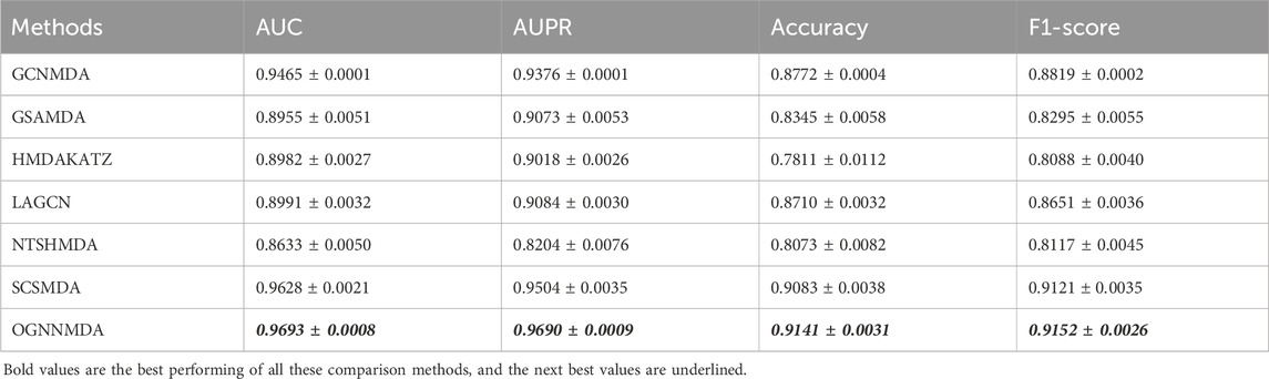
Table 2. Comparison of AUC, AUPR, Acc, and F1-score obtained by each method based on aBiofilm dataset at 5-cv.

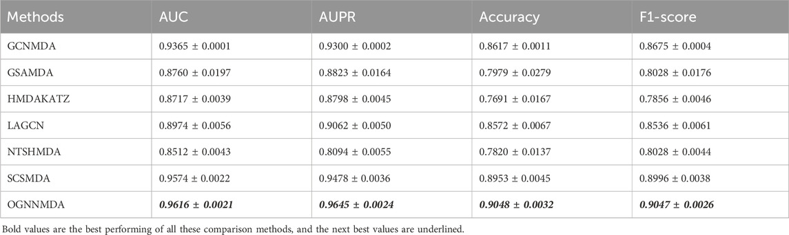
Table 3. Comparison of AUC, AUPR, Acc and F1-score obtained by each method based on MDAD dataset at 5-cv.

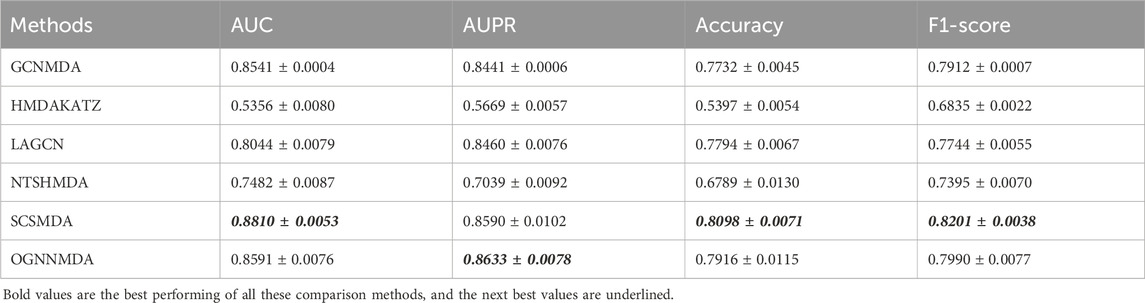
Table 4. Comparison of AUC, AUPR, Acc and F1-score obtained by each method based on DrugVirus dataset at 5-cv.

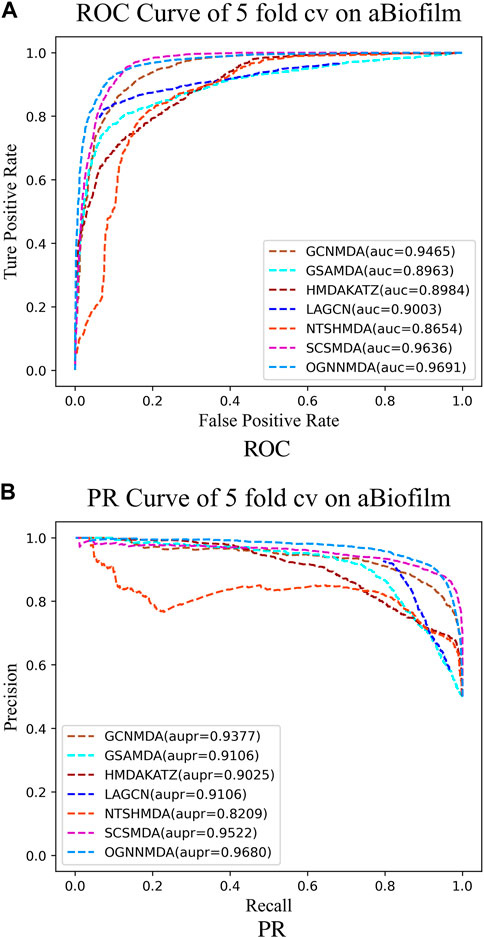
Figure 4. (A) ROC curves for each modeling approach based on the aBiofilm dataset 5-cv. (B) PR curves for each modeling approach based on the aBiofilm dataset 5-cv.

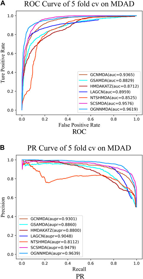
Figure 5. (A) ROC curves for each modeling approach based on the MDAD dataset 5-cv.