
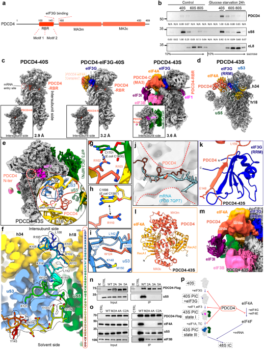
記住我

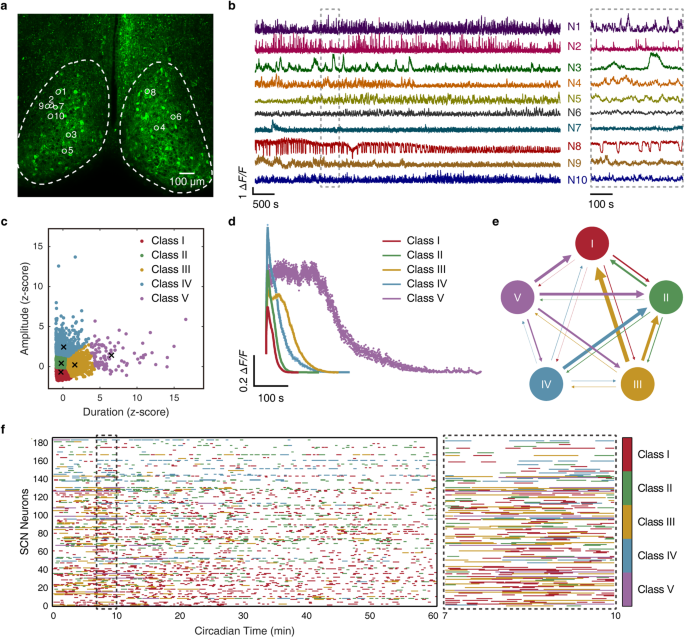

We applied two-photon microscopy to image freshly isolated SCN slices from adult Viaat-Cre::GCaMP6f mice with their GABAergic neurons expressing the genetically coded Ca2+ indicator GCaMP6f. To capture temporal properties of different scales, time-lapse images were acquired at 2.7 Hz for 6 h without any interruption (Fig. 1a). In all GCaMP6f-expressing neurons, transient, discrete Ca2+ events, namely Ca2+ bursts, occurred atop slow baseline Ca2+ oscillations (Fig. 1b). Intriguingly, SCN Ca2+ bursts varied drastically by virtue of frequency, amplitude, duration and, in rare cases, polarity; their waveforms were polymorphic, being spiky, or triangle-shaped with a slow descending slope, or echelon- or square-shaped with a conspicuous plateau (Fig. 1b). When Ca2+ bursts were categorized by a K-means clustering algorithm based on duration and amplitude, we identified five classes of Ca2+ bursts as determined by the gap statistic method (Supplementary information, Fig. S1a),18 with average durations spanning from 17.4 s to 129 s at 5% and 95% percentiles (Fig. 1c, d; Supplementary information, Fig. S1b, c). The frequency of Ca2+ bursts in the SCN neuronal population displayed a broad bell-shaped distribution, ranging from 0.001 Hz to 0.011 Hz at 5% and 95% percentiles; and the inter-Ca2+ burst intervals followed a roughly exponential distribution with a long tail (Supplementary information, Fig. S1d, e). Notably, the vast majority of neurons underwent frequent switching between different classes of Ca2+ bursts, with a tendency being switched to classes of shorter duration (Fig. 1e, f; Supplementary information, Fig. S1f). This result suggests that Ca2+ bursts of distinctive classes likely constitute fundamental units to form higher-order temporal features for time representation and computation in the SCN.
Fig. 1: Multiscale Ca2+ activities in SCN GABAergic neurons.
a A representative two-photon image showing GABAergic neurons expressing GCaMP6f in an SCN slice from an 8-week-old Viaat-Cre::GCaMP6f mouse. Dashed lines demarcate the estimated borders of the SCN. Scale bar, 100 μm. b Diversity of SCN neuronal Ca2+ signals. Data shown are 1-h excerpts from a total of 6-h continuous recording at a 2.7 Hz frame rate, and corresponding neurons are marked in a. Right, an enlarged view of the segment in the dashed box. c Clustering of Ca2+ bursts based on their duration and amplitude by a K-means clustering algorithm. Crosshairs mark the centroid of 5 classes identified. d Time courses of averaged Ca2+ bursts in different classes. Data are shown as mean ± SEM (n = 4643, 3150, 764, 638, and 100 events for class I, II, III, IV, and V, respectively). e Schematic diagram of inter-class switching of Ca2+ bursts. The direction and relative thickness of the arrow represent the direction and relative propensity of switching, respectively. f Raster plot showing the kinetics of inter-class switching of Ca2+ bursts. Right, an enlarged view of the segment in the dashed box.
Encouraged by these observations, we sought to investigate population-level Ca2+ activity in the entire SCN over an intact circadian period. However, we met with an unforeseen challenge that two-photon microscopy can penetrate SCN only to the depth of ~200 μm at a tolerable laser intensity. To overcome this limit, we designed and custom-built a dual-view two-photon microscope, both inverted and upright, doubling the penetration depth and fluorescence collection efficiency while lowering photodamage. The perfusion system was also adapted for temperature control, sterilization, and dual-side perfusion of the slice over a prolonged culture time (Supplementary information, Fig. S2). Meanwhile, to improve the signal-to-noise ratio, we opted to use Viaat-Cre::GCaMP6s mice for brighter fluorescence signals.19 Using this system, we performed time-lapse volumetric imaging of 650 μm × 650 μm × 300 μm SCN slices at 0.67 volumes/s for 5-min recording every hour up to 30 h, and obtained six complete datasets (Supplementary information, Table S1). In a typical volume stack, we extracted Ca2+ time series from 6000–9000 neurons along with their spatial coordinates, via a custom-devised image analysis pipeline (Supplementary information, Fig. S3).
As judged from the kinetics of inter-class switching of Ca2+ bursts, we assumed that an SCN neuron stays at the same functional state within a short time period (e.g., 5-min). It follows that the ensemble of all 5-min recordings collected from thousands of neurons over a circadian period shall cover virtually all Ca2+ states attainable by SCN GABAergic neurons. To this end, we resorted to machine learning technology to develop an automated Ca2+ state classifier. We first transformed Ca2+ time series into phase-space manifolds,20,21,22 and summarized them into six states contingent on visual observation (Fig. 2a–c). Subsequently, we constructed and trained a graph convolutional network (GCN)23,24,25 to assign Ca2+ states to individual neurons based on their 5-min Ca2+ behavior (Supplementary information, Fig. S4). The simplest manifold came from State I (0.60% in total), showing a ring-shaped structure, while the most complex manifold came from State II (0.84% in total), showing a three-pointed star. The predominated state, State VI (93%), exhibited fast, irregular, and nonperiodic fluctuations in the time domain, and gave rise to a stochastic oscillating manifold in the phase space, whereas State V was the rarest (0.04%, Fig. 2d) and characterized by brief downward deflections from consistently elevated Ca2+ levels. When mapped to the SCN space, all these minority states entwined irregularly and the mosaic pattern variably evolved at different circadian times (Fig. 2e; Supplementary information, Fig. S5).
Fig. 2: Ca2+ states and state-switching dynamics in SCN neurons.
Data were from a slice containing 6049 identified neurons. a Representative 5-min Ca2+ recordings, corresponding to different Ca2+ states of SCN neurons (State I to State VI). Data shown are Z-score normalized fluorescence intensity. b, c Phase-space manifolds (b) and recurrent plots (c) of corresponding traces in a. Note the repeating features or motifs of systematic dynamics in the recurrent plot. d Percentage of neurons at different Ca2+ states over a 24-h timescale. See Supplementary information, Fig. S4 for neuronal Ca2+ state classification. e Spatial distribution of neuronal Ca2+ states at CT28. The most populous State VI neurons (inset, top right) are omitted for clarity. f Raster plot of state-switching over 24 h for all neurons. The color codes of Ca2+ states are shown on the right.
Over a 24-h period, while waxing and waning through different Ca2+ burst classes, most neurons also displayed robust inter-state switching behavior (Fig. 2f), hinting at the existence of even higher-order temporal features of Ca2+ signals. Indeed, when Ca2+ signal amplitude (mean ΔF/F over a 5-min recording) was analyzed as a function of time, we revealed significant differences between two 12-h divisions, i.e., high-activity Ca2+ mode (H-mode) and low-activity Ca2+ mode (L-mode) over a 24-h period. Such circadian Ca2+ rhythmicity was confirmed in almost all SCN neurons examined, along with neuron-to-neuron variability in the timing of inter-mode transition (Supplementary information, Fig. S6).
Notably, a dramatic event switching to State IV occurred around circadian time (CT) 30 (Fig. 2f). By reviewing this event in the SCN space, we identified an SCN-wide activity, namely phase wave of hyperactivity (PWHA), which originated from the peripheral SCN, entered the SCN at the dorsal tip (CT26), then propagated to the ventromedial region (CT28–CT29), triggered a global Ca2+ excitation (CT30) before fading out (CT31–CT38) (Supplementary information, Fig. S7 and Video S1). This finding is consistent with previous reports on extremely slow Ca2+ waves in cultured neonatal SCN.10,16 The observation that PWHA lasted on a 12-h timescale and swept across the entire nucleus indicates that it represents a spatiotemporal feature of the largest scales in the SCN.
Taken together, we uncovered a full spectrum of multiscale Ca2+ events at the SCN neuronal and ensemble levels, ranging from elemental Ca2+ bursts (seconds to minutes) to Ca2+ states (minutes to hours) to Ca2+ modes as well as population-level PWHA (~12 h). This finding underscores the idea that time-keeping by SCN is much more sophisticated than simply maintaining global coherent oscillations via synchronization.
Ensemble Ca2+ signals predict hourly timeTo investigate whether and how multiscale SCN Ca2+ signals encode and decode time information, we quantified neuronal and ensemble Ca2+ behaviors in relation to physical time. We reckoned that, as Ca2+ signals are intimately related to SCN inputs and outputs, understanding the time-keeping principles of the SCN can be naturally cast as learning the feature representation of the multiscale Ca2+ activity.
Taking all observed neurons in each SCN as a whole, we employed principal component analysis26,27,28 to appraise the collective properties of all the 5-min Ca2+ time series in a low-dimensional space. We found that the resultant data points in the PC1–PC2 space delineated a circular temporal evolution trajectory (Fig. 3a). This result inspired us to further explore whether one could utilize SCN Ca2+ signals to predict physical time and, in so doing, highlight the SCN’s core function as a time-keeping system.
Fig. 3: Hourly time prediction by polling randomly selected cohorts of SCN neurons.
a Circular evolution trajectory of a 2D representation of population-level Ca2+ activities. Axes correspond to the first two principal components, PC1 and PC2. Different time points are represented in different colors, and consecutive time points are connected by dotted lines. b Scheme of time-predictor based on SCN Ca2+ signals. Conv and FC refer to the convolutional and fully connected layer; N, T and D denote the dimensions of neurons, the input Ca2+ time series of each neuron and its features extracted, respectively. c Accuracy and loss curves during training process. d Prediction accuracy curves, showing results from six SCN slices. Data are shown as mean ± SEM (n = 5000 trials). Lower dashed line represents the chance level. e Visualization of CNN’s high-dimensional features in a 2D space via t-SNE. From left to right: the number of neurons is 1, 100, 300, and 900, respectively.
We therefore employed modern deep learning tools29,30 to decode time information from SCN Ca2+ signals. Using a convolutional neural network (CNN) consisting of one convolutional layer, a residual block followed by one fully connected (FC) layer, we achieved hourly time prediction by involving randomly selected cohorts of neurons (Fig. 3b, c). To be specific, single-neuron Ca2+ signals could predict the correct time at a slightly above-the-chance level, supporting their ability of time feature representation. Prediction accuracy steeply increased with the size of the cohorts polled and reached 99.0% ± 0.4% (mean ± SEM, n = 6) at a cohort size of 900. Even higher accuracy of time prediction could be attained by polling a still greater number of neurons (Fig. 3d). To confirm that such discrimination of time truly reflects disparities hidden in the Ca2+ time series, we visualized the output features of the second convolutional layer in a two-dimensional (2D) space via t-distributed stochastic neighbor embedding (t-SNE).31 Clearly, as the cohort size increased, the data points gradually congregated into distinctive clusters in the feature space, and became more compact within clusters and more separable between clusters (Fig. 3e). Thus, hourly time prediction by SCN is contingent on the integration and computation of Ca2+ signals from cohorts of neurons, analogous to group decision-making in a statistical system.
Next, we estimated the contribution coefficient for each and every neuron from the integrated gradient-based attribution map after min-max normalization.32 Histograms of contribution coefficients of individual neurons were well fitted to a Gaussian distribution, at all time points examined (Supplementary information, Fig. S8a), while for a given neuron, its contribution coefficient fluctuated over time (Supplementary information, Fig. S8b). However, after being averaged over an intact circadian period, single-neuron contribution coefficient exhibited a very narrow Gaussian distribution, with a mere 7% difference between the 5% and 95% percentiles (Supplementary information, Fig. S8c). Thus, our quantitative assessment suggests that, on a 24-h scale, all SCN neurons contribute uniformly in terms of time computation.
Modular time representation in the SCNClassic topological division of the SCN is based on retinal and efferent connectivity and expression of neuropeptides, with VIP/GRP in the ventral “core” region and AVP in the dorsal “shell” region.33,34 Regional oscillators in the SCN, namely the evening oscillator and the morning oscillator, and the light-responsive area exhibit photoperiodic changes in response to different external photoperiods.35,36 Recently, single-cell RNA-sequencing has allowed for fine-grained cell type classification, identifying five SCN neuron subtypes occupying distinct spatial domains.37 To identify functional organization patterns hidden in the ensemble Ca2+ behavior of SCN, we cast the problem of functional neuron subtype classification as time-series representation learning in an unsupervised manner, and built a classifier TraceContrast (Fig. 4a). In this classifier, we leveraged contrastive learning,38 a cutting-edge unsupervised machine learning paradigm, in which Ca2+ time series augmented with transformations such as masking and cropping (i.e., positive samples) were contrasted against those from different timestamps or neurons (i.e., negative samples) in a hierarchical fashion. By enforcing the consistency among features of positive samples, TraceContrast should be able to capture emergent properties of SCN Ca2+ signals that are invariant to transformations.
Fig. 4: Modular time feature representation revealed by TraceContrast.
a Scheme of neuron subtype classification by TraceContrast. N, T, and D denote the dimensions of neurons, the input Ca2+ sequence of each neuron and its output features, respectively. b Bilaterally symmetric and hierarchical modularity emerged from neuron subtype classification. The predefined number of clusters (K) is listed below each corresponding image. c The t-SNE plots of the dimensionality reduction corresponding to b. d Time predictability when sampling only within one specific module (K = 5). Lower dashed line represents the chance level. Data are shown as mean ± SEM (n = 5000 trials). Note that one-module-only sampling results in a marked disruption to time prediction accuracy compared to random sampling in all SCN neurons. Similar results were obtained when K = 2, 3, 4. e, f Ca2+ signal amplitude and corresponding variance (e) and average MIC in different modules (f). Data are shown as mean ± SEM (n = 1587, 1936, 1211, 835, and 480 for Modules 1, 2, 3, 4 and 5, respectively). Note that the two attributes showed smooth inter-modular gradients running in opposite directions.
By TraceContrast, we categorized all observed neurons from the same SCN slice into 2, 3, 4, or 5 functional subtypes (Fig. 4; Supplementary information, Fig. S9). Using t-SNE to visualize the learned high-level features, we found that the clusters were well separated after their dimensionality reduction into 2D space (Fig. 4c). Spatial mapping revealed that same-type neurons aggregated in the SCN space, giving rise to distinctive ripple-like patterns with bilateral symmetry (Fig. 4b; Supplementary information, Video S2). With an increasing number of subtypes, fine-grained modules were peeled off layer by layer in a coherent and continuous manner, indicating a modular and hierarchal time feature representation by Ca2+ signals in the SCN.
We tested the robustness of modular organization in the SCN. We showed that PWHA appeared to exert no effects on the modular organization for two reasons. Firstly, the diffusion direction of the modular ripple did not align with that of PWHA. Secondly, by division of the 24-h Ca2+ sequence into three 8-h segments, with no PWHA in the first segment, the modular ripple remained intact for all three subsets of data, affirming that it is indeed PWHA-independent (Supplementary information, Fig. S10a–c). By spatial and temporal subsampling, we showed that, albeit noisier, the bulk of the modular ripple was unchanged when only 50% of neurons were retained by the farthest point sampling method39 (Supplementary information, Fig. S10d) or when every other data point in 5-min recordings were dropped out (Supplementary information, Fig. S10e). Furthermore, symmetric modular ripple emerged even from single-sided analysis using either left or right SCN data independently. Altogether, we conclude that the modular ripple-like organization is an emergent property pertaining to time feature representation by the SCN at work.
Using the time predictor described above, we demonstrated that single-module sampling resulted in a markedly degraded performance as compared with random sampling across all modules (Fig. 4d). To further explore topological specificity, we generated module-specific time predictors by training each of them with data from one module only. We showed that the accuracy attainable for same-module time prediction was still greater than 99%, but its cross-module time prediction ability was almost completely abolished (Fig. 5), suggesting that each module has a full yet unique representation of time features.
Fig. 5: Module-specific time predictors and their performance.
Dataset was the same as in Fig. 4 with K = 3. Three module-specific time predictors were trained, each using data from the pertinent module, and its performance pertaining to hourly time prediction was tested in all 3 modules, in order to assess their same-module and cross-module time predictability. The lower dashed line in each panel represents the chance level. Data are shown as mean ± SEM (n = 5000 trials).
To gain insight into the nature of invariant properties captured in contrastive learning, we analyzed module-specific Ca2+ signal amplitude and variance, and uncovered their ordered variation over modules, manifesting as a smooth ventrolateral-to-dorsomedial upward gradient (Fig. 4e). We also measured the maximal information coefficient (MIC),40,41 an index of the coupling strength within a module. While changing dynamically over time, MIC also exhibited an ordered spatial gradient, except that it ran in the opposite direction (Fig. 4f). In other words, our neuron subtype classification might have captured Ca2+ signal attributes and coupling strength as invariant properties.
留言 (0)