Penetrating microelectrodes have proven invaluable in neurophysiological studies, allowing for the recording [1–4] and stimulation [5–8] of neural activity. They have also shown promising results in neuroengineering applications, particularly in the field of neuroprosthetics [9–11]. For example, in visual cortical prosthetics, intracortical microstimulation (ICMS) delivered through implanted probes in the visual cortex has been extensively used to investigate evoked neural responses [12–14], animal behaviors [15–18], and even restore some aspects of visual perception and perceived visual experiences in human subjects [19–23]. In terms of the downside of penetrating microelectrodes, the longevity of recording and stimulation performance [24] and the potentially linked tissue reactions like gliosis around electrodes [25] have been explored. These studies not only provide new insights into the electrophysiological properties of cortical networks but also underscore the need for additional studies to enable successful applications of future visual prosthetic devices. In order to make progress towards these applications, a deeper understanding of the underlying mechanisms that govern the spatiotemporal properties of neuronal activation by different ICMS parameters is crucial. Despite significant advancements [26–32], there are still numerous gaps in our understanding of the stimulation paradigm, as the parameter space associated with ICMS is vast. Many aspects of the interactions between ICMS and local networks also remain largely unexplored.

While many studies have examined the activation of neuronal responses induced by ICMS, fewer studies have characterized the depressive effects of ICMS on the neural response following stimulation [6, 31, 33–35]. Previous research has demonstrated significant depression of neural activity following single or repetitive ICMS, occurring at various time scales ranging from milliseconds to hours. However, due to variations in recording methods and stimulation parameters, there is still a lack of comprehensive understanding of this depression phenomenon. In the context of sensory restoration, such as visual prostheses, it is crucial to consider the critical frequencies of sensory cortical neurons that can enable continuous sensory perception. Exploring whether refractory periods, neuronal depression, adaptation, or active inhibition contribute to the loss of activation in response to ICMS [36] remains an open area for investigation. Developing a better understanding of ICMS-induced depression will facilitate innovations in controlling this effect to ultimately enhance prosthetic performance.

Emerging imaging tools are providing novel insights into ICMS-induced activation and depression, improving traditional technologies like electrophysiology by capturing activity from populations of neurons with spatial information. Concurrent measurements of tissue oxygenation can help determine whether neuronal depression results from metabolic mismatch [37]. Neuronal activation is typically followed by changes in blood supply, altering local oxygen delivery. Intrinsic optical imaging, sensitive to the oxidative state of hemoglobin, provides a convenient method for obtaining these measurements. Additionally, intrinsic imaging aids in distinguishing between bulk fluorescence decreases resulting from increases in hemoglobin absorption and those caused by decreases in calcium ion (Ca2+) concentration. Establishing a quantitative relationship between the evoked neuronal response and oxy-/deoxy-hemoglobin hemodynamic signals is essential for estimating oxygen extraction and consumption (metabolic load) vs. stimulation-induced fatigue caused by ICMS [38].

Here, we conducted quantitative analyses of neuronal Ca2+ activity and hemodynamic responses to various ICMS frequencies and visual stimulation in Thy1-GCaMP6s mice, which expressed genetically-encoded Ca2+ indicator (GCaMP6s) in excitatory neurons [39] using in vivo mesoscopic-scale widefield fluorescence and intrinsic imaging. In addition, we also examined somatic and neuropil responses to ICMS in vivo with high-resolution two-photon microscopy. We compared the Ca2+ and hemodynamic responses between ICMS and visual stimulation conditions. Our findings revealed that visually-evoked Ca2+ responses exhibited balanced magnitudes of activation and depression. However, electrically-induced Ca2+ responses were dominated by activation, which was frequency-dependent. We observed that hemodynamic responses persisted beyond the period of Ca2+ activation extending into the post-stimulus depression phase. Furthermore, our two-photon Ca2+ imaging demonstrated that the 25-Hz ICMS resulted in the most pronounced activation and depression, particularly in the soma, but depression was also observed at higher frequencies. These findings indicate that neuronal depression resulting from stimulation-induced reduction in neuronal excitability exhibits a distinct frequency preference compared to activation. This depression effect demands a high energy supply and has a relatively stronger impact on the activated region compared to visual stimulation. Taken together, these results provide novel insights into microstimulation-induced neural activity, which can contribute to the advancement of ICMS strategies for numerous applications including intracortical sensory prostheses.

2.1. Animals and surgery

Transgenic mice expressing the Ca2+ indicator in excitatory neurons (Thy1-GCaMP6s; 024275, Jackson Laboratory, ME, USA) were used for simultaneous recordings of Ca2+ and hemodynamic signals under the mesoscopic-scale microscopy (n = 8) and for two-photon Ca2+ imaging (n = 9) studies. Surgical procedures were conducted following previously established protocols [27, 30, 31]. Briefly, mice were anesthetized with a mixture of xylazine (7 mg kg−1 b.w., i.p.; Covetrus, OH, US) and ketamine hydrochloride (75 mg kg−1 b.w., i.p.; Covetrus). Craniotomies were then performed over the left visual cortex (AP = −1 to −5, LM = 0.5–3.5 mm). Custom stimulation microelectrodes (Q1x4-3mm-50-703-CM16LP, NeuroNexus Technologies; single 3 mm-long shank, 30 µm-diameter four channels, 50 µm site spacing, electrochemically activated iridium/iridium oxide sites [40]) were implanted at an angle of 20–30° slanted towards the posterior region. The electrode was securely fixed to the skull with UV-curable resin (e-on Flowable A2, BencoDental, PA, USA). Reference and ground lines on the electrode connector were wired to the bone screws placed in the skull over the frontal lobes. Kwik-Sil was used to fill the exposed cortical surfaces in the craniotomy to maintain visibility, and a cover glass was used to seal the craniotomy with UV-curable resin. Anesthesia level was periodically monitored and an update (ketamine, 45 mg kg−1 b.w., i.p.) was administered as necessary. Throughout the surgical procedure and recovery period, the mice's body temperature was maintained using a heating water pad and respiration was monitored visually. Following surgery, antipamezole hydrochloride (Antisedan, Zoetis, NJ, US; 1 mg kg−1 b.w., i.p.) and ketoprofen (Ketofen, Zoetis; 5 mg kg−1 b.w., i.p.) were administered for reversal of anesthesia and for analgesia. After recovery, mice were allowed to recover for up to 2 h prior to the recording session. Animals were kept in a 12 h/12 h light/dark cycle. All procedures described here were approved by the Division of Laboratory Animal Resources and Institutional Animal Care and Use Committee at the University of Pittsburgh and performed in accordance with the National Institutes of Health Guide for Care and Use of Laboratory Animals.

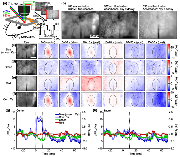
2.2. Mesoscopic and microscopic image acquisition

Animals were placed in a custom treadmill and head-fixed throughout the imaging experiments. We employed a mesoscopic-scale widefield microscope (MVX-10 epifluorescence microscope; Olympus, Tokyo Japan; 6.3× zoom) for simultaneous recording of Ca2+ and intrinsic optical signals over a relatively larger field-of-view of 2.3 mm × 1.7 mm (figure 1(a)). The imaging was conducted with three sequentially interwoven LED illuminations, and barrier filters were placed in front of each LED light source to restrict the spectral band of each LED to the desired wavelength: (1) blue for GCaMP6s excitation (482.5 ± 15.5 nm; #67-028, Edmund Optics Inc., NJ, US); (2) green for measuring hemoglobin-sensitive imaging (532 ± 2 nm; FLH532-4, Thorlabs Inc., NJ, US); and (3) red for differentiating oxy- and deoxy-hemoglobin (633 ± 2.5 nm; FLH633-5, Thorlabs Inc.) [37, 41]. Fluorescence and reflectance intensities were collected through a long-pass filter (>500 nm; ET500lp, Chroma Technology Corporation, VT, US) placed in the emission path before the camera (QImaging Retiga R1; Cairn Research Ltd, Kent, UK) and images were sampled at 30 Hz (10 Hz for each color). The camera was controlled using Micro-Manager software [42, 43] with an imaging matrix size of 344 × 256 pixels (figures 1(b)–(e)).

Figure 1. Mesoscopic-scale widefield imaging of Ca2+ and hemodynamic signals. (a) The experimental setup involved applying a widefield single-photon excitation of GCaMP (483 nm) and hemodynamic-visualization illumination (532 and 633 nm) to the mouse cortex (i) and acquiring mesoscopic-scale fluorescent and reflectance images (ii) during ICMS (iii). (b) Example images taken with different colored light sources. GCaMP fluorescence image with 483 nm excitation light (left), total hemoglobin absorbance image with 532 nm illumination (middle), and deoxyhemoglobin-dominant absorbance image with 633 nm illumination (right). (c)–(f) Raw and change-ratio (0–30 s from the 10 Hz ICMS onset) images with blue (c), green (d), and red (e) illuminations. Blue corresponds to uncorrected Ca2+ signals. Vessel patterns are visible in these images. (f) Hemodynamic correction of Ca2+ signal attenuates reductions on the vessel patterns. (g) Four different time courses of uncorrected Ca2+, corrected Ca2+, green, and red signals simultaneously recorded in the 10 Hz ICMS condition within a center region (dotted ellipse in (c)–(f), 400 µm in horizontal and 600 µm in vertical axes from the stimulation site). The hemodynamic correction shifts the Ca2+ signals upward during and after the stimulation period. (h) Time courses in the entire imaging field. Scale bars = 500 µm.

Download figure:

Standard image High-resolution image

Two-photon microscopy (Bruker, Madison, WI, US) was performed using a laser tuned to 920 nm wavelength (Insight DS+, Spectra-Physics, Menlo Park, CA) for GCaMP6s excitation (laser power ≈ 10–20 mW, figure 11(a)). Resonant Galvo scanning was performed to capture higher resolution images at 30 Hz over a 413 × 413 µm2 field of view (512 × 512 pixels) at a single z-plane focused around the stimulation site. In both imaging conditions, each recording was composed of a 30 s pre-stimulation period, a 10 s stimulation period, and a 60 s post-stimulation period.

2.3. Electrical (ICMS) and visual stimulation

ICMS was performed using an IZ2 stimulator controlled by an RZ5D base processor (Tucker-Davis Technologies, FL, US). Each pulse consisted of a 200 µs cathodic leading phase followed by a 200 µs anodic phase, with balanced charges between the cathodic and anodic phases. The current was fixed to ±20 µA (4 nC/phase), selected to be lower than the safety limit (k = log(Q) + log(Q/A) ≈ 0.36 < 1.7, where Q and Q/A represent charge per phase [µC/phase] and charge density per phase [µC cm−2/phase], and value k below 1.7 can be considered as a safe configuration [44]). Six different train frequencies (10, 25, 50, 100, 250, and 500 Hz) were tested. The order of ICMS trials was repeated two times in ascending-descending frequency order (10–500, 500–10, 10–500, 500–10 Hz).

For comparison, a single blue LED was positioned in front of the animal's eye contralateral to the imaging window as a more natural visual stimulus (n = 5 out of 8 mice in the mesoscopic-scale widefield imaging, n = 5 out of 9 mice in the two-photon imaging). The LED was controlled by the stimulator, applying a square wave at 10 Hz (50 ms on, 50 ms off, 50% duty cycle) with an amplitude of 2.5 V. All stimulation trials were repeated 4 times.

2.4. Analyses and statistics2.4.1. Pre-processing of the widefield and two-photon imaging data

Analyses were performed using custom-made scripts written in Python (ver. 3.9, Python Software Foundation, DE, US) along with existing modules: numpy, scipy, scikit-image, statsmodels, and matplotlib. The frames of image stacks were preprocessed through spatial binning (to 20 µm/pix for the mesoscopic-scale widefield imaging, and to 1 µm/pix for two-photon imaging) and temporal binning (to 2 Hz) with anti-alias filtering to enhance signal-to-noise ratio. Image registration was conducted on each frame to align them to the first frame of each acquisition by cross-correlation with sub-pixel estimation. For the two-photon microscopy images, additional inter-line alignment was applied as necessary to correct for shearing between lines.

For the widefield imaging data, masks were generated to exclude blood vessels from further analyses (figure S1). Average images from each color (blue, green, and red) were intensity-threshold binarized using hysteresis thresholding with the following two threshold levels: (i) mean-0.5 standard deviation (SD) and (ii) mean-1SD. Spatially connected vessel patterns were extracted after the hysteresis thresholding. A pixel-wise logical summation of all color channels was then calculated to combine them and generate the final vessel pattern image. This procedure also captured pixels on probe shanks that exhibited noticeably low fluorescence and reflectance values.

2.4.2. Somatic region of interest (ROI) definition for the two-photon imaging data

Response images of excitatory neurons acquired under the two-photon microscopy were constructed by calculating pixel-wise mean fluorescent change ratio during the stimulation period (0–10 s) over pre-stimulation mean fluorescent intensity across the entire imaging region. For each animal, these response images for all stimulation conditions were averaged. ROI for each soma was manually defined with Fiji [45].

2.4.3. Neuronal Ca2+ response quantification for widefield and two-photon imaging

To quantify the excitatory Ca2+ activity for two-photon imaging, the fluorescence change ratio (dF/F0 = (F(t) − F0)/F0) was calculated, where F(t) represents the fluorescent intensity at time t and F0 is the mean fluorescent intensity over the pre-stimulation period (−30 ⩽ t < 0, in s).

In the case of the mesoscopic-scale widefield imaging, the Ca2+ signals were corrected based on the green channel values to account for the hemodynamic effect that could potentially affect the green GCaMP signals [37, 41] (figures 1(f)–(h)). The corrected dF/F0(t) was calculated using the formula:

where represents the reflectance intensity to the green illumination at a specific time point t, and is the mean of the reflectance intensity to the green illumination during the pre-stimulation period.

2.4.4. Hemodynamic activity quantification of mesoscopic-scale widefield imaging

The change in oxy- and deoxy-hemoglobin concentrations relative to baseline ( and , respectively; the solution for the modified Beer–Lambert law) were calculated as follows [37]:

where constant represents the absolute absorption spectra of HbR and HbO at 532 and 633 nm, constant represents the pathlengths at wavelength l (i.e. l = 532 and 633 nm). Il(t) and Il,0 are the reflectance intensities at a time point t and its mean value during the pre-stimulation period for wavelength l. The values of and were obtained from [37], and if an exact wavelength value was not provided, the mean value of the adjacent two values was used.

The change in the total hemoglobin concentration () was calculated by summing the changes in oxy- and deoxy-hemoglobin (). The oxygen extraction fraction (OEF; relative concentration of deoxyhemoglobin in total hemoglobin concentration) was estimated using the following:

where [HbR]0 and [HbT]0 represent baseline concentrations of the deoxyhemoglobin and total hemoglobin. For our estimations, we assumed baseline concentrations of 2 mM for hemoglobin in blood, 3% of blood in brain tissue (60 µM of total hemoglobin), and 75% of oxygenation (15 µM of deoxyhemoglobin) [37]. By definition, real OEF values range between 0 and 1. Therefore estimated OEF values outside this range were excluded as outliers (2.4 ± 1.0% pixels, mean ± SD across all animals).

2.4.5. Extraction of significant activation and depression in the widefield imaging data

To define activation and depression distances (from stimulation site), latencies (onset timing), and durations (offset timing–onset timing) of the spatiotemporal magnitude profile of the corrected dF/F0, Δ[HbO], and Δ[HbR] while reducing the effect of data fluctuations, we employed hysteresis thresholding. As described above, this method requires two different threshold levels [46]. First, the original three-dimensional data (dF/F0, Δ[HbO], and Δ[HbR]) obtained under the mesoscopic-scale imaging (X × Y × time) was converted into two-dimensional structure (distance from stimulation site × time). We calculated the mean ± 1 and 2 SDs of the pre-stimulation period (−30–0 s), and used them as the soft and hard thresholds. To determine the activation distance, we identified points on the distance profile with values above 2 SDs as well as points between 1 and 2 SDs that were connected to distances above 2 SDs as above threshold. The same procedure was applied in the time domain, resulting in a joint threshold image (distance × time) that contained multiple continuous regions. The regions extracted by the hysteresis thresholding were considered candidates for significant activation and depression. We selected at most one region for each activation and depression event based on specific criteria. For activation candidates in ICMS experiments, we selected single regions that (1) emerged within 10 s after stimulation onset, (2) occurred within 50 µm from the stimulation site, and (3) had the longest duration among the candidates. For depression candidates in ICMS conditions, we selected single regions that (1) emerged within 20 s after stimulation onset, (2) occurred within 50 µm from the stimulation site, and (3) had the longest duration among the candidates. Similarly, for visual stimulation conditions, we used criteria (1) and (3) regardless of whether the responses originated from the inserted probe. The onset timing of the extracted region is defined as latency, and the difference between onset and offset timings is duration. Activation and depression distances and mean amplitude across the distance are represented as functions of time from stimulation onset.

After defining the distance, latency, and duration of significant Ca2+ activation or depression and hemodynamic activities (d[HbO] and d[HbR]) using the hysteresis thresholding method described above, these measurements were averaged across time for each mouse (e.g. symbols in figure 4(d)). Also, the averaged measurements for each mouse were averaged across mice to evaluate these effects as a function of stimulation conditions such as ICMS frequencies and visual stimulation (e.g. bars in figure 6).

The balance of activation and depression was quantified using the following metrics: distance from the stimulated site, response magnitude, and response duration. Balance based on these metrics was calculated as follows:

where Mact and Mdep represent metrics for activation and depression, respectively. The resulting score ranged from −1 (biased to depression) to 1 (biased to activation); 0 indicated balanced activation and depression.

2.4.6. Statistical procedures

For pair-wise comparisons, we conducted t-tests on two-related samples (e.g. figure 3(c)). One-way and two-way analysis of variance (ANOVA) were used for a comparison among three (or more) groups. For example, in figure 5(a), we compared neural activation distances across different stimulation conditions using one-way ANOVA, and in figure 9(a), we compared response distances across stimulation conditions and signal modalities using two-way ANOVA. Post-hoc analysis was performed using Tukey's honestly significant difference (HSD) test. To quantify correlations between signals from shared units (e.g. between dF/F0 values in % or |%| in figure 5(h)), the Pearson correlation coefficient was used. For correlations involving signals with different units (e.g. between dF/F0 in % and oxyhemoglobin concentration in µM in figure S4(e)), we used Spearman's rank correlation coefficient. Statistical significance was evaluated based on a significance level of p< 0.05. Significant results are denoted by asterisk symbols in the figures or summarized in tables. In cases where there were samples without significant activation and/or depression, the metrics such as magnitude and duration were replaced with zero in the statistical analyses of the two-photon imaging data.

In this study, we investigated the spatiotemporal dynamics of excitatory neurons, focusing on their activation and depression, using 10 s ICMS trains at various frequencies and compared those to visual stimulation. These experiments were conducted using widefield imaging and two-photon microscopy. We quantified the magnitude, spatial extent, latency, and duration of the excitatory neuron responses as well as the induced oxyhemoglobin and deoxyhemoglobin signals. Throughout this paper, we refer to 'depression' as the phenomenon in which the neural Ca2+ signal decreases in intensity due to stimulation compared to the pre-stimulus period.

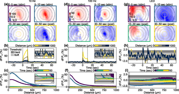
3.1. ICMS elevates excitatory Ca2+ activity followed by post-stimulus depression

Although stimulation-induced depression of neuronal excitability (SIDNE) has been previously described [34], most imaging studies have focused on stimulation-induced activation [5, 26, 29, 47]. To investigate the extent of spatiotemporal activation and depression, we first analyzed ICMS-induced changes in Ca2+ activity within excitatory neurons using widefield imaging. We first show results from a representative animal to highlight the spatio-temporal changes (figure 2; see movies S1–S3 for entire frames). A 10 s long ICMS train at 10 Hz was delivered to the visual cortex and produced a clear increase in Ca2+ activity during the stimulation period, which spread to approximately 500 µm away from the stimulation site (0–10 s; figures 2(a)–(c)). Following the cessation of the stimulation train (at 10 s), the Ca2+ activity rapidly declined and dipped below pre-stimulus baseline ('depression') approximately 5 s after the ICMS offset (figure 2(b)) and persisted for several tens of seconds during the post-stimulation period although with a noticeably smaller magnitude than activation. This depression effect was particularly prominent in the region exhibiting an increase in Ca2+ (figure 2(c)). The Ca2+ data were corrected for hemodynamic absorption (as shown in figures 1(f)–(h)) to mitigate this potential signal source. Similar patterns of activation and depression were also observed with 100 Hz ICMS (figures 2(d)–(f)), but no such effects were observed during visual stimulation (figures 2(g)–(i)), where the visual stimulation train induced transient activation at the onset and offset periods. Visually-evoked activation and depression spread through almost the entire imaging field due to the use of uniform visual field stimulation.

Figure 2. Activation followed by depression of Ca2+ responses induced by stimulation. (a), (d), and (g) Single-animal examples of colormap in the X–Y domain during (a) 10 Hz ICMS, (d) 100 Hz ICMS, and (g) visual stimulation. Concentric circles indicate distances from the stimulation site, plotted at 250 µm intervals. Asymmetric color scales were used for enhanced visualization. (b), (e), and (h) Time courses of the Ca2+ responses to (b) 10 Hz ICMS, (e) 100 Hz ICMS, and (h) visual stimulation at various distances from the stimulation site. Line colors correspond to ones of concentric circles in (a), (d), and (g). Light and dark gray areas indicate pre-stimulation fluctuations (mean ± 1SD and mean ± 2SD) used for the hysteresis thresholding. Vertical dotted lines indicate stimulation onset (t = 0 s) and offset (t = 10 s). Horizontal dotted lines indicate pre-stimulation baseline (dF/F0 = 0). Insets indicate enlarged time courses (scalebars for x and y axes = 10 s and 1%, respectively). (c), (f), and (i) Temporal changes in distance profiles of Ca2+ response to (c) 10 Hz ICMS, (f) 100 Hz ICMS, and (i) visual stimulation. Line colors correspond to ones of panel frames in (a), (d), and (g). Vertical dotted lines indicate half of the probe width (27.5 µm), where data points are excluded due to vessel masking. Insets indicate enlarged distance profiles (scalebars for x and y axes = 100 µm and 1%, respectively).

Download figure:

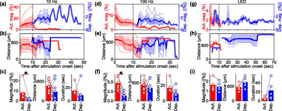
Standard image High-resolution image

The magnitude, duration, and distance of activation and depression were quantified for each animal. The Ca2+ responses induced by the 10 Hz ICMS across all animals (figures 3(a)–(c)) showed that the average magnitude of Ca2+ activation increased over time, while the average magnitude of Ca2+ depression remained relatively low and constant (figure 3(a)). Since Ca2+ depression emerged in the distal region from the stimulation site (figure 2(a); see results 3.5) and prolonged Ca2+ activation remained around the center region, these temporal periods of Ca2+ activation and depression partially overlapped. The activation distance remained constant throughout the ICMS train, followed by varying degrees of depression distance ranging from 300 to 1000 µm away from the stimulation sites (figure 3(b)). Activation was observed in all mice (8/8 mice), while depression was observed in most cases (5/8) (see methods 2.4.5 for definition of activation and depression). Although the depression magnitude was attenuated by the hemodynamic correction (paired t-test, t = 1.75, p = 0.12), it was significantly greater than zero (one-sample t-test, t = 3.03, p < 0.05; figure S2(a)). The depression component in the uncorrected Ca2+ signals was significantly stronger than the change observed in the green channel (paired t-test t = 3.00, p < 0.05; figure S2(b)). These observations show that the hemodynamic correction works sufficiently with our data and the Ca2+ depression remained even after the hemodynamic correction, meaning that the depression was not a feint due to hemodynamic signal contamination.

The Ca2+ activation was significantly stronger than the depression by almost an order of magnitude (comparison of absolute magnitude; figure 3(c), left; t = 3.22, p< 0.05). However, there was no statistical difference in the mean distances between activation and depression (figure 3(c), middle; t = 1.29, p= 0.24). The duration of the activation tended to be longer than the duration of depression (figure 3(c), right; t = 1.22, p= 0.26). It is worth noting that the Ca2+ activation lasted slightly longer than the 10 s stimulation period. These results indicate that the 10 s, 10 Hz ICMS train consistently evoked sustained activation throughout the stimulation period, followed by depression to a similar spatial extent. These trends were highly dependent on the stimulation parameters and modalities, where 100 Hz ICMS induced transient activation that was stronger than depression in magnitude (figures 3(d)–(f), t = 7.97, p < 0.05), and visually-induced activation was comparable to depression (figures 3(g)–(i), t = 1.07, p = 0.34).

Figure 3. Population analyses of Ca2+ activation and depression induced by stimulation. (a) Temporal dynamics of Ca2+ activation (red, left vertical axis) and depression (blue, right vertical axis) magnitudes under 10 Hz ICMS condition. Each pale line indicates an individual mouse. Thick lines and shaded areas indicate mean ± 1SD. (b) Temporal dynamics of the activation (red) and depression (blue) distances under 10 Hz ICMS condition. ((c), left) Comparison of mean magnitudes between the activation and depression under 10 Hz ICMS condition. ((c), middle) Comparison of mean distances between activation and depression under 10 Hz ICMS condition. ((c), right) Comparison of durations between the activation and depression under 10 Hz ICMS condition. (d)–(f) Same metrics evaluated under 100 Hz ICMS condition. (g)–(i) Same metrics evaluated under visual stimulation condition.

Download figure:

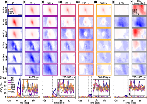
Standard image High-resolution image 3.2. ICMS frequencies modulate Ca2+ activation and depression

Given that ICMS-induced activation is followed by depression of the Ca2+ response, we then asked how the stimulation frequencies can impact features of the induced activation and depression of the Ca2+ response (figure 4). In a representative animal, we observed activation-dominant responses to the ICMS where lower-frequency stimulation induced an elevating (or sustained) response and higher-frequency stimulation elicited a transient and localized response. Similar profiles were also observed in all mice (8/8 mice). Meanwhile, the visually-evoked response exhibited transient activation and depression with similar magnitudes (5/5 mice with visual stimulation). These representative examples of the excitatory neural Ca2+ responses provide valuable inspiration about the complex interactions between stimulation frequencies and their effects on the Ca2+ response.

Figure 4. Frequency dependency of ICMS-Induced responses and comparison with visual-evoked response. (a)–(f) Responses to ICMS with various frequencies. (First and second rows): transient (first row) and sustained (second row) phases during the stimulation period. (Third to sixth rows): Transient (third row) and sustained (fourth to sixth rows) phase after the stimulation train offset. Scale bar = 500 µm. (g) Response to 10 Hz LED blink stimulation to the contralateral eye. The color scales in (a) to (g) are the same for comparison. (h) Response to the visual stimulation shown with a magnified color scale for better visibility. (i) Time courses of the ICMS-induced and visual responses at different distances from the stimulation site (left to right: 0–250, 250–500, 500–750, and 750–1000 µm). Insets show the responses around the onset and offset of the stimulation train (vertical dotted lines, 10 s) with a magnified y scale (scale bar = 1% dF/F0; horizontal dotted line = 0%).

Download figure:

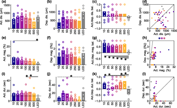
Standard image High-resolution image 3.3. Ca2+ activation and depression prefer different ICMS frequencies

Given the observed frequency-dependent relationship between the magnitude, area, and spatiotemporal aspects of ICMS-induced activation and depression, we conducted further analysis to quantify the differences between stimulation conditions and examine the correlations between activation and depression (figure 5). We determined the response distances and durations of significant activation and depression using the hysteresis thresholding of the mesoscopic-scale Ca2+ spatiotemporal dynamics (see Methods 2.4.5). Neither the activation nor depression distances showed any statistical differences among the stimulation conditions (figure 5(a), activation, one-way ANOVA, F = 1.71, p= 0.14; figure 5(b), depression, F = 1.50, p= 0.20). The balance of the activation and the depression distances (equation (6) did not differ among the stimulation conditions (figure 5(c), one-way ANOVA, F = 0.65, p= 0.69). Furthermore, we did not observe any significant correlations between the activation and the depression distances (figure 5(d)).

Figure 5. Frequency dependency of the activation and depression distance, magnitude, and duration among various ICMS frequencies and visual stimulation. ((a) and (b)) Activation (a) and depression (b) distances. For the ICMSs, the longest-lasting Ca2+ response that occurred within 10 s (for activation) and 20 s (for depression) after the stimulation onset, within 50 µm from the stimulation site was extracted. For the visual stimulation, the criterion of stimulation site coverage was not applied. (c) Balance between activation and depression distances (equation (6)). (d) Correlation between activation and depression distances for each animal. ((e) and (f)) Activation (e) and depression (f) magnitudes. (g) Balance between activation and depression magnitudes. (h) Correlation between activation and depression magnitudes. ((i) and (j)) Activation (i; horizontal dotted line = 10 s stimulation duration) and depression (j) durations. (k) Balance between activation and depression durations. (l) Correlation between activation and depression durations. * with solid line indicates p < 0.05 for pairwise comparison using post-hoc Tukey's HSD test ((a)–(c), (e)–(g), and (i)–(k)), * with dashed line indicates p < 0.05 for one-way ANOVA without post-hoc pairwise significant difference. Colored * indicates p < 0.05 for Pearson correlation coefficient in corresponding conditions ((d), (h), and (l)).

Download figure:

Standard image High-resolution image

Although the area of ICMS-induced activation did not differ significantly, the magnitudes of activation were significantly different among the stimulation conditions (figure 5(e), one-way ANOVA, F = 3.10, p< 0.05). Lower-frequency ICMS tended to induce stronger activation, while the visual stimulation tended to elicit weaker activation compared to ICMS (post-hoc Tukey's HSD test, 10 Hz ICMS vs visual stimulation, difference = −6.6%, p< 0.05). In contrast, the magnitudes of depression were not statistically different across all stimulation conditions (figure 5(f), one-way ANOVA, F = 1.39, p= 0.24). Consequently, the balance between these two magnitudes were significantly different among the stimulation conditions (figure 5(g), one-way ANOVA, F = 7.02, p< 0.05), with visual stimulation showing balanced activation and depression responses (post-hoc Tukey's HSD test, 10 Hz ICMS vs visual stimulation, difference = −0.75, p< 0.05; 25 Hz ICMS vs visual stimulation, difference = −0.52, p< 0.05; 50 Hz ICMS vs visual stimulation, difference = −0.56, p< 0.05; 100 Hz ICMS vs visual stimulation, difference = −0.52, p< 0.05; 250 Hz ICMS vs visual stimulation, difference = −0.61, p< 0.05; 500 Hz ICMS vs visual stimulation, difference = −0.67, p< 0.05). Moreover, the magnitudes of activation and depression exhibited significantly strong positive correlation in the 10, 50, and 100 Hz ICMS conditions (figure 5(h); Pearson correlation coefficient, 10 Hz ICMS, r = 0.73, p< 0.05; 50 Hz ICMS, r = 0.82, p< 0.05; 100 Hz ICMS, r = 0.75, p< 0.05). These findings indicate that ICMS at lower frequencies elicits stronger Ca2+ activation in excitatory neurons, while visual stimulation induces a balanced response of activation and depression. Additionally, the correlations of magnitudes between activation and depression suggest that there may be shared or related mechanisms underlying the processes of activation and depression in certain ICMS conditions.

The activation durations were significantly dependent on the stimulation conditions (figure 5(i), one-way ANOVA, F = 2.36, p< 0.05). All ICMS frequencies, particularly around 100–250 Hz, caused prolonged activation that lasted beyond the duration of the stimulation train (10 s, horizontal dotted line in figure 5(i)). In contrast, visual stimulation only caused transient activation at the onset and offset of the stimulus train (post-hoc Tukey's HSD test, 100 Hz ICMS vs visual stimulation, difference = −11 s, p< 0.05; 250 Hz ICMS vs visual stimulation, difference = −12 s, p< 0.05). Here, we quantified a static aspect of activation based on the thresholding (see Methods 2.4.5), which also extracted weak sustained activity. However, as shown in the representative example (figure 4), stimulation frequency and modality also modulated the activation in a different way, especially in terms of peak magnitudes at each time point (e.g. higher-frequency ICMS induced transient activation). This dynamic aspect is further investigated in the later section (see Results 3.4).

Similar to activation, the duration of depression varied depending on the stimulation conditions (figure 5(j), one-way ANOVA, F = 2.48, p< 0.05), with tendencies of longer depression at 25–50 Hz ICMS and visual stimulation compared to the other conditions (no significant pairwise difference by post-hoc Tukey's HSD test). Consequently, the balance between the activation and depression durations exhibited significant dependence on the stimulation conditions (figure 5(k), one-way ANOVA, F = 4.77, p< 0.05). Depression tended to be longer in the 25 Hz ICMS and visual stimulation compared to the other conditions, while activation dominated in the lower and higher-frequency ICMS conditions, especially at 500 Hz (post-hoc Tukey's HSD test, 10 Hz ICMS vs visual stimulation, difference = −0.89, p< 0.05; 25 Hz ICMS vs 500 Hz ICMS, difference = 0.71, p< 0.05; 250 Hz ICMS vs visual stimulation, difference = −1.00, p< 0.05; 500 Hz ICMS vs visual stimulation, difference = −1.08, p< 0.05). No significant correlation was found between the duration of activation and depression (figure 5(l)). These results suggest that ICMS at any frequency entrains the Ca2+ activity, while the degree of subsequent depression is dependent on the stimulation conditions. Together, these quantitative findings inform the selection of stimulation frequencies, where the neural responses include both activation and depression phenomena.

3.4. Different ICMS frequencies evoke different spatiotemporal dynamics of Ca2+ activation

Since it was observed that lower-frequency ICMS caused greater sustained Ca2+ activation, while higher-frequency ICMS caused transient and localized activation followed by weak sustained activation (figure 4(i), leftmost panel, 2–10 s), we proceeded to investigate how activation developed during the stimulation train across different conditions (figure 6). In the 10 Hz ICMS condition, the activation gradually increased in magnitude over the 10 s ICMS duration and spread through the visual cortex. On the other hand, in the 100 Hz condition, the Ca2+ activity initially peaked, and then decreased over the 10 s ICMS duration, becoming more localized (figures 6(a)–(d)).

Figure 6. Temporal dynamics of the activations. ((a) and (b)) Response maps (a) at 0–2, 2–4, 4–6, 6–8, and 8–10 s after the stimulation onset and line profiles in the medio-lateral axis around the stimulation site (b) at 0–2 (blue) and 8–10 s (green) in response to the 10 Hz ICMS. Scale bar in (a) = 500 µm. Horizontal and vertical scale bars in (b) = 500 µm and 10%, respectively. The Inset in (b) shows the same profiles normalized to each peak value. ((c) and (d)) Response maps (c) and line profiles (d) in response to the 100 Hz ICMS. (e) Examples of activation distance (top) and speed (bottom) during the stimulation period in the 10 and 100 Hz ICMS conditions. Positive and negative speeds indicate expansion and shrinkage of activation distance, respectively. (f) Population activation distance (top) and speed (bottom) (mean ± 1SD). (g) Speed averaged across animals (mean ± 1SD). (h) Examples of the activation magnitude (top) and change rate (bottom). A positive change rate indicates growing-up activation magnitude. A change rate of zero indicates constant activation magnitude. (i) Population magnitude (top) and change rate (bottom) (mean ± 1SD). (j) Magnitude change rate averaged across animals (mean ± 1SD). * with line indicates p < 0.05 for pairwise comparison with post-hoc Tukey's HSD test ((g) and (j)).

Download figure:

Standard image High-resolution image

To quantify the spatiotemporal dynamics of neural Ca2+ activation, we measured the distance from stimulation site to activation edge at each frame and calculated the spread/withdrawal speed based on the inter-frame difference of the distance (0.5 s interval). For the 10 Hz condition, the activation distance remained relatively stable over the 10 s ICMS period, resulting in a near-zero spreading speed (figure 6(e)). In contrast, the activation distance rapidly decreased after 2 s of the 100 Hz ICMS, leading to a negative speed (withdrawal of activation) observed 4–5 s after the onset. The