This observational, longitudinal study analyses data from a more extensive project, approved by the local ethics committee (Comitato Etico Milano Area 2; 568_2018bis) on fall risk assessment in neurological patients at discharge from rehabilitation. The primary study’s results on fall risk have been recently published [25].

Inclusion criteria were:

Age over 65 years;

Affected by one of the following neurological syndromes: hemiparetic gait secondary to a stroke, peripheral neuropathy of the lower limbs or parkinsonism secondary to a vascular encephalopathy or Parkinson’s disease.

Informed consent to participate in the study.

With respect to the exclusion criteria:

Presence of two neurological diagnoses (e.g. hemiparesis and Parkinson’s disease);

Inability to complete the TUG test and the 10 m walking test without touching assistance on admission or discharge;

Completing any of the mobility tests using an assistive device (e.g. a cane, a walking frame) on admission or discharge;

Completing the TUG test in more than 30 s on admission or discharge;

Severe visual impairment or hearing loss.

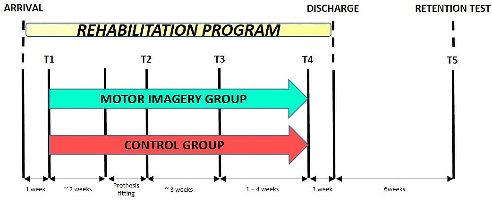
Assessment

Participants completed two assessment sessions, the first at the beginning (T0) and the second at the end (T1) of the rehabilitation program (Fig. 1). In each session, a detailed balance and gait assessment was administered. In the current study, only data from the 10 m walking test and the TUG test are reported.

Fig. 1

Time course of the mobility assessment. Gait and balance have been assessed in two assessment sessions, T0 and T1 (dark grey boxes), the first at the beginning and the second at the end of the participants’ inpatient rehabilitation stay (light grey box). Five repetitions of the 10 m walking and TUG tests have been collected in each session. Trial2 − 3 is constituted of repetitions 2 and 3 while Trial4 − 5 by repetitions 4 and 5. Measures of the variable of interest from a single test repetition are referred to here as “metric” (e.g. the five repetitions of, say, the 10 m walking test return five metrics of gait speed). Participants’ measures are given by the mean of two metrics (e.g. participants’ gait speed measures from Trial2 − 3 are the mean of the gait speed metrics from repetitions 2 and 3) or by the median of all five repetitions. Horizontal arrows: time, expressed in days and minutes for the upper and lower drawings, respectively

A physiotherapist or an occupational therapist administered both tests, and both the 10 m walking test and the TUG test were repeated five times in each session. Participants completed the TUG test with an inertial measurement unit (mHT-mHealth Technologies, Bologna, Italy) attached to their lower trunk.

In the 10 m walking test [26], participants were asked to walk straight while a clinician measured with a stopwatch the time taken to walk the central six meters of a 10 m long trajectory.

The conventional three m TUG test [11] was administered as follows. Participants were asked to wait for a go signal from the experimenter and then stand up from a chair, walk in a straight line, turn around a traffic cone, return to the chair and sit down. Trunk acceleration and angular velocity along the three axes were recorded by the inertial sensors. In addition, the experimenter measured the TUG test duration (TTD) with a stopwatch.

The 10 m walking and TUG tests were completed at the patient’s comfortable speed.

In our previous works, the five test repetitions were analysed individually, mobility metricsFootnote 1 were collected from each, and their median value was used as the patient’s mobility measure (e.g. [12, 27,28,29]). Here, instead, persons’ measures were obtained from two repetitions, a full-fledged shortened version of the five repeats mobility tests. This choice was taken to calculate more accurate LMMs for SEM estimation (i.e. maximal models [30] with random intercepts and slopes, see below). As a preliminary step, the measurement accuracy of the reduced tests was compared to our previous measurement reference (i.e., the five repeats tests).

The gait speed (m/s) was calculated for each 10 m walking test repetition, and from each TUG test repetition the following were collected:

1.

TUG test duration (TTD, s),

2.

Sit-to-walk (STW) duration (s),

3.

Turning duration (i.e. the duration of the first turning phase; s),

4.

Peak angular velocity along the vertical axis during turning (ω, °/s).

For the reduced versions of the walking and TUG tests, the first of the five repetitions was considered a “test ride” (e.g. the patient gets confidence with the test set), thus being discarded.

Metrics from repetitions 2 and 3 (which together form Trial2 − 3) are averaged, and these average values are called Trial2 − 3 measures. Similarly, metrics from repetitions 4 and 5 are averaged and referred to as Trial4 − 5 measures.

It is worth stressing that in the reduced versions of the walking and TUG test set up here, a single participant’s measure (e.g., the participant’s gait speed and TTD) comes from two test repetitions. Hence, in each session, two participants’ measures were collected. As explained below, Trial4 − 5 is used to assess the stability of the Trial2 − 3 measures.

The inertial measurement unit software automatically returned the STW, turning duration, and ω metrics for each test repetition [31].

StatisticsAssessing the agreement between the reduced and the five-repeat mobility tests

The agreement between the measures from the reduced versions of the walking and TUG tests and those from the complete tests (i.e. the five-repeat tests) was assessed with the method-comparison analysis [32], popularised by Bland-Altman [33], and the absolute percentage error (APE).

In the Bland-Altman analysis run in the current study, the x-axis reported the full test measures, i.e. the reference measures. On the y-axis was the difference between the measures from the reduced test measures and the reference measures.

The reduced test measures are considered a good approximation of the criterion standard if the Bland-Altman analysis shows no bias and the limits of agreement are sufficiently narrow: the absence of bias indicates that the new measures are accurate; the tight limits of agreement suggest that these are precise.

Acceptable limits must be defined a priori [34], and deciding if the limits of agreement are sufficiently tight depends on what the new measure is used for [35]. This indication is recommendable and relatively easy to implement for widely used measures such as gait speed and TTD. However, judging the maximum tolerable amplitude of the limits of agreement is more challenging for newer, less investigated measures, such as those from the inertial sensors.

For this reason, APE was also calculated as follows:

$$APE=100\times \left|\frac\right|$$

(1)

With \(N\): new measure (here the measures from the reduced tests, i.e. Trial2 − 3 measures), \(R\): reference measure (here the measures from the five repeat tests, i.e. the reference measures).

The APE 95th percentile (APE95%) was chosen as an agreement indicator.

SEM estimation with linear mixed-effects models

In the Classical Test Theory (CTT) framework, a single measure is the sum of the true quantity of the measured variable plus the measurement error. Under the assumption of (i) random, (ii) uncorrelated errors and (iii) errors uncorrelated with the true value of the measured variable, the variance of measures (i.e. the observed variance, in the CTT jargon) results from the sum of the true and error variances [4, 36].

The ANOVA is commonly used to disentangle the different sources of variation, with variance estimates derived from ANOVA mean square values [5, 37].

In particular, the total variance is modelled from the sum of the between-subjects mean square and the within-subjects mean square, with the within-subjects mean square equalling the error variance [5]. In this regard, SEM is simply the square root of the error variance [4].

As an alternative to ANOVA, linear mixed-effects models (LMMs) [38] can decompose the variance in different sources and isolate the measurement error variance [20].

LMMs are an invaluable statistical method for the analysis of complex datasets, such as those, common in medicine, made of contrasting groups of participants (e.g. patients vs. controls; patients receiving different treatments) assessed repeatedly in time (e.g. before and after treatments).

The formula of an LMM has three parts, one for handling fixed effects, another for random effects and a third consisting of an error term.

The fixed effects are used to represent sources of systematic variation in the data. In the regression jargon, the fixed effects correspond to the predictors.

Random effects account for variations within clusters, accounting in this way for an amount of variance of the response variable which is not explained by the fixed effects. For example, random effects can be used to model the variability of a cluster of non-independent measures, such as repeated data collected by an individual at a time point.

Finally, LMMs also contain an error term, which accounts for the residual variance not explained by the fixed or random effects.

Consider a clinical trial in which patients are randomized into two treatment groups and assessed three times. In each assessment session, multiple measures are collected from each participant, a common approach to address measurement error and obtain robust person estimates.

In the LMM framework the patient’s group (e.g. treatment A vs. treatment B), the assessment session (e.g. before, immediately after treatments and at follow-up) and the group × session are modelled as fixed effects. Random effects would be here the subjects, modelled as random intercepts and, in a maximal model [30], the assessment session, modelled as random slopes.

In this example, LMMs would be used for significance testing and an Analysis of Variance could be run on the LMM showing, say, that the response variable is significantly improved after treatment compared to before.

To put it simply, the fixed effect returns the average improvement in the response variable in the sample after treatments. The random intercept component specifies that each participant has a unique baseline value for the response variable and the random slope that each participant can improve to a different extent at the treatment end (i.e. that each participant has their slope of improvement).

In addition to significance testing, LMMs can also be used for prediction or, as done here and mentioned above, for variance decomposition to estimate the standard error of the measurement. This last application of LMMs is still unconventional and will be better developed in the following paragraphs.

Among the strengths of LMMs, in addition to the aforementioned ability to manage data not independent of each other, there is their robustness to missing data and the possibility they offer to easily control for confounding effects [37].

The participants recruited in the current study received physiotherapy and occupational therapy between the two assessment sessions. Indeed, they completed a rehabilitation program to improve their balance and gait. In line with our former findings [27, 28], it is reasonable to expect that, on average, the patient’s gait and balance at T1 were likely better than at T0. This fact violates the “steady-state assumption”, i.e., that the patient does not evolve, which is fundamental to SEM estimation in CTT [21].

In a typical CTT study in which a clinical measure’s reliability and SEM are calculated, subjects are measured twice, usually one or two weeks apart. This time interval between the two measurements is considered long enough to prevent recall but short enough not to change the “true” value of the measured variable [39]. In this scenario, it can be reasonably assumed that the true value of the variable remains the same in the two sessions. Any difference in measurement between the two sessions can then be attributed only to the measurement error.

LMMs provide a suitable solution if the steady-state assumption is not valid [21]. The idea is straightforward. Therapeutic exercise is expected to improve gait and balance in neurological patients, thus causing a change between T0 and T1 in the variables of interest and measures. By using LMMs, this change in time can be estimated and removed: the steady state is created mathematically.

In the current study, the following LMM model was used to estimate SEM of measurement Y (say Y is TTD, but the next holds for any of the mobility measures considered here):

With \(_\), the predicted TTD for session \(s\) and individual \(i\);

\(_\), the TTD baseline level (i.e. the model’s intercept); the TTD at T0, when the predictor equals zero;

\(_\), the random intercept component, indicating the deviation from \(_\) for subject \(i\);

\(_\), the session effect (i.e. the model’s slope); the change in TTD associated with a predictor’s change;

\(_\), the random slopes component, indicating the deviation from \(_\) for subject \(i\);

\(_\), the predictor variable, here session, which takes values 0 for T0 and 1 for T1;

\(_\), the residuals, calculated for each \(i\) in each session \(s\).

The model also specifies that \(_\), \(_\) and \(_\) are normally distributed, have mean equals zero, and each their variance. In particular, \(_\) variance is labelled \(^\). Moreover, LMMs also consider the covariance between \(_\) and \(_\).

Including the random intercepts and slope terms allows the model to consider two clinically essential aspects.

First, it is unrealistic that all participants have the same TTD at baseline (i.e., that \(_\) is the same for all participants). Instead, it seems more likely that at T0, they are distributed around an average value.

Second, it is equally unrealistic for a participant to change the same after the rehabilitation (i.e., that \(_\)is the same for all). Even if unexpected, some individuals could worsen, for example, due to the occurrence of a complication. Moreover, even if all persons would improve, the amount of improvement (i.e. the responsiveness to rehabilitation) is likely to be different in different patients.

When LMMs are used for estimating SEM, it is assumed that deviations in the observed measure from the model’s prediction (i.e. the model’s residual) are caused by the measurement error. Hence:

And once SEM has been estimated, the 95% MDC can be calculated as customary:

$$95\% MDC=1.96\times \sqrt\times SEM$$

(4)

It is worth stressing that, according to Eq. (2), the measured variable (in the example the TTD) depends, and only depends, on the assessment session (i.e. if it has been collected in T0 or T1) and the person being evaluated (and the estimated random effects variances and covariances and residuals variance). Any additional, unmodeled source of variation that moves the observations away from the model’s predictions and causes an increase in residuals is included in the residual variance.

The following will make this last point clear. In the current study, in each assessment session, two trials were repeated. It can be reasonably assumed that the quantity of the variable of interest, say TTD, does not change within a session (in a sense, a within-session steady-state assumption holds). Therefore, any difference in measures from Trial2 − 3 and Trial4 − 5 can be attributed to measurement error.

However, the LMM Eq. 2 does not explicitly model TTD as affected by the trial. In other words, the trial is not considered a source of TTD variation and any trial effect on TTD remains unquantified. Instead, any within-session difference in the measures from Trial2 − 3 and Trial4 − 5, a difference attributed to the measurement error, would be included in the residual variance of model 2.

Complying with the linear mixed-effects models’ assumptions

Equation (2) LMM relies on two assumptions: residuals are normally distributed and have constant variance. Therefore, when built on LMMs, SEM and MDC also rely on these assumptions.

Quantile-quantile plot and the absolute residuals plot as a function of the predicted values are used here to assess residuals’ normality and homoscedasticity. If these are violated, the response variable is ln-transformed. Notably, if the predictor is ln-transformed, the MDC obtained from the LMM is meant to be applied to ln-transformed measures.

Say that ω needs to be ln-transformed and that a patient improved their peak angular velocity during turning at rehabilitation end. This improvement is a real improvement if:

$$\text}__}- \text}__}>MDC$$

This inequality can be rearranged as follows:

$$\text\left(\frac}__}}}__}}\right)>MDC$$

$$\frac}__}- }__}}}__}}>^-1$$

Therefore, when the measure is ln-transformed, the MDC can be understood as the baseline measure’s minimum percentage change exceeding the measurement error.

Longitudinal agreement between the 95% MDCs and the “all five repetitions better than the best” method

We have previously proposed a method, referred to in the current study as “all five repetitions better than the best”, which is considered here the reference method to determine if a patient’s mobility measure has improved (or worsened) after rehabilitation [28]. According to this method, a participant improved if all five repetitions in the T1 session were better than the best repetition in T0. Conversely, if all five repetitions in the T0 session were better than the best repetition in T1, the participant got worse.

The accuracy of the 95% MDC was assessed by evaluating their agreement with the “all five repetitions better than the best” method. Since the agreement between these two methods is about the change of the patients in time, it will be referred to as a “longitudinal agreement” to avoid confusing it with the cross-sectional agreement assessed in the previous analyses.

Two indices have been used to assess longitudinal agreement: the weighted Cohen’s kappa and Youden’s J.

For Cohen’s kappa analysis, participants were classified as improved, stable and worsened according to the 95% MDC (Trial2 − 3 measures) and the reference method.

Cohen’s kappa is a chance-corrected agreement measure [40]. The weighted variant (squared weights) considers that disagreement can have different seriousness. For example, consider a patient flagged as improved by the reference methods but indicated as stable by the 95% MDC. If the 95% MDC had identified this patient as worsened, it would have been a more severe error.

While the intuition behind chance-corrected agreement methods is valuable, Cohen’s kappa can give paradoxical and unreliable results with some datasets. For this reason, it has been recommended that the results of a complementary analysis, essentially based on sensitivity and specificity, are presented alongside Cohen’s kappa [41]. Youden’s J [42] was calculated here for this purpose.

Participants were dichotomised into stable and changed (i.e. significantly got better or significantly got worse) according to the 95% MDC and the reference method. The number of true and false positives and negatives is counted (e.g. true positives: number of participants that changed their status according to the 95% MDC and the reference method), and Youden’s J is calculated.

Youden’s J ranges from 0 to 1 (with 1 meaning there are no false positives or negatives) and can be interpreted as the probability of correctly classifying a patient (i.e., correctly identifying a changed patient or a stable patient) penalised by the chance of making an error.

SEM estimation from reliability indices from the subset of steady participants: a control analysis

According to the previous analysis, participants can be divided into changed (i.e. participants who improved after rehabilitation or, less likely, who got worse) and stable (i.e. participants who did not change between sessions with respect to the variable of interest).

Patients who did not change represent a pool of individuals for whom the steady-state assumption holds. CTT reliability indices and the corresponding SEM can be calculated on this subset of participants and compared to the SEM returned by the LMM analysis.

For this complementary analysis, stable participants were defined according to the complete five repetitions tests (i.e., the reference tests), similarly to what was done in the longitudinal agreement analysis but applying stricter criteria.

A single participant was considered stable, i.e. the steady-state assumption was verified in them in the case of the following:

$$\left[\text\left(_\right)> \text\left(_\right) \right] \& \left[\text\left(_\right)< \text\left(_\right)\right]$$

With \(\text\left(_\right)\), the maximum value of the variable on the five repetitions collected in session T0 (remaining symbols alike). Of course, the steady-state assumption also held if the opposite occurred.

In other words, stable participants are those for which the two extreme repetitions (e.g. the shortest and the longest TTD, the fastest and the lowest for gait speed) in a session (i.e. T0 or T1) are more extreme than the two extreme repetitions in the other session (i.e. T1 or T0).

Once the subset of unchanged participants was constituted, the Intraclass Correlation Coefficient (ICC) was calculated as the CTT reliability index.

A two-way mixed effect, absolute agreement (i.e. including systematic and variable error), single measurement model was used in this analysis as recommended for assessing test-retest reliability [43, 44]. Note that this model, nomenclature according to McGraw and Wong [18], corresponds to ICC2,1 of Shrout and Fleiss [19] from a strict computational point of view [5].

Only Trial2 − 3 measures from T0 and T1 have been considered for the ICC calculation.

To correspond with the primary analysis, ICC2,1 has been chosen over alternative models, such as ICC2,k.

As previously mentioned and as done elsewhere, e.g. [45]. , two metrics from two test repetitions were averaged to provide a single measure in this study. This one measure was used then as the response variable in the LMMs for the primary analysis. Hence, these measures were also included in the ICC models in place of the original metrics. Since a single measure was obtained from two metrics, a single-measurement, absolute agreement ICC model was chosen.

About the choice of ICC2,1, it is also worth noting that the mobility measures used here are, in a way, composite measures precisely because they are derived from two preliminary metrics. In this scenario, computing the ICC2,1 is similar to calculating the ICC2,1 of questionnaire total scores, where the questionnaire total score is the one measure that is derived from many metrics (i.e. the questionnaire items).

It should also be stressed that the subset size can differ for the different measurements and is the smallest for the measure with the highest responsiveness to rehabilitation [27, 28].

A sums of squares approach (i.e. ANOVA) was used for reliability estimation rather than regression (i.e. LMMs) to stay more in line with the CTT framework.

After estimating reliability, the SEM was calculated according to:

$$SEM=__}\times \sqrt$$

(5)

With \(__}\), the standard deviation of the T0 measures.

Finally, the 95% MDC was obtained per Eq. (4).

All analyses were run in R version 4.2.3 “Shortstop Beagle” (The R Foundation for Statistical Computing). The library “lme4” [46] was used for fitting LMMs. Type 1 error probability was set at 0.05 and corrected in post hoc tests, according to Holm [47]. As done for the SEM estimation, when used for hypotheses testing, LMMs assumptions were assessed, and the response variable was ln-transformed if needed.