The design and outcomes of the BLISS-LN study (GSK Study 114054; NCT01639339) have been reported previously [15, 16]. In brief, BLISS-LN was a Phase 3, double-blind, placebo-controlled, 104-week study that evaluated the safety and efficacy of belimumab 10 mg/kg IV plus background standard therapy in adults with active LN. The study was conducted across 107 sites; all sites received approval from their respective ethics committees or institutional review boards.

During the BLISS-LN study, blood samples were collected for PK analysis of belimumab serum concentration at the following time points: 0, 3, 14, 28, 56, 168, 171, 364 and 728 days. Urinalysis (proteinuria measured by urine protein/creatinine ratio [uPCR]) and hematology assessments were performed at baseline and every 4 weeks for the duration of the study.

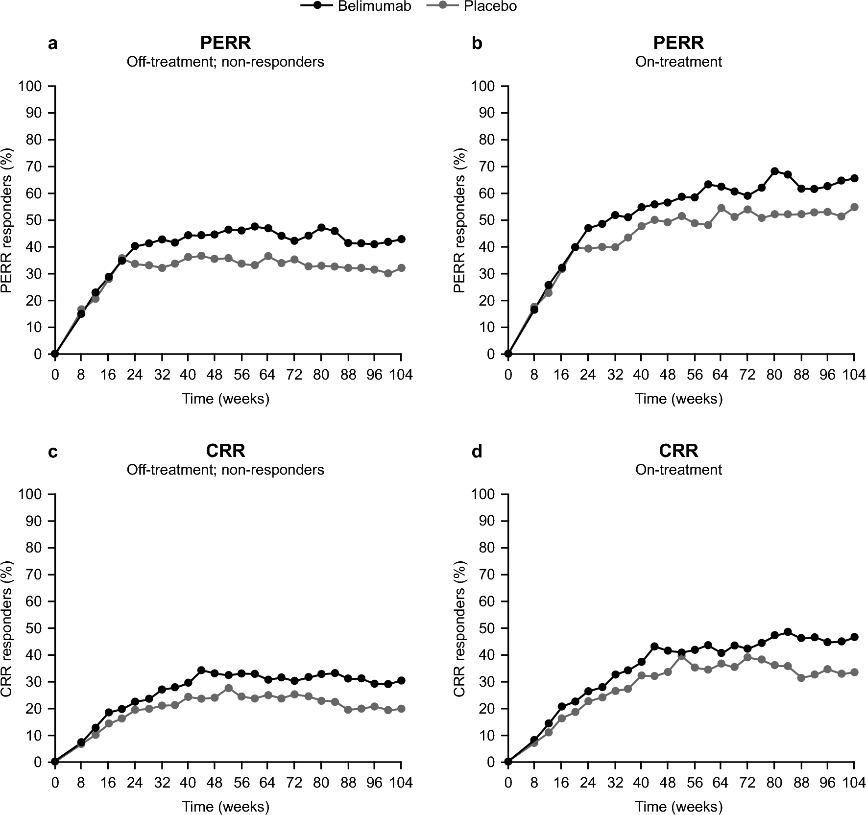
In this longitudinal analysis, the dichotomous PERR and CRR data from BLISS-LN were analyzed. A PERR responder was defined as a patient with an estimated glomerular filtration rate (eGFR) no more than 20% below the pre-flare value or ≥ 60 ml/min/1.73 m2 of body surface area, with uPCR ≤ 0.7 (g/g), and who had not received rescue therapy. The more stringent CRR was defined as an eGFR of no more than 10% below the pre-flare value or ≥ 90 ml/min/1.73 m2 of body surface area, with uPCR < 0.5 (g/g), and who had not received rescue therapy. If the PERR/CRR responder criteria were not met, patients were classified as non-responders as per a composite variable estimand strategy.

A longitudinal logistic model of the responder probability was fitted to individual efficacy response data collected over time from the placebo and active arms of the BLISS-LN study, for each efficacy endpoint (PERR or CRR) separately. Specifically, the model was defined as:

Equation 1: Longitudinal logistic model for PERR or CRR responder rate

$$Logit\left(_(t)\right)=_ - _\bullet ^}}_\bullet t}+_\times }$$

where: PRESP(t) is the probability of response at time t, RRSS defines the responder rate at steady state in placebo, ∆RR defines the overall change in the responder rate from baseline to steady state in placebo, KRR is the rate constant for the change in responder rate over time, and θBEL is the effect of belimumab therapy on the responder rate. TRT is a binary variable (0 for placebo, 1 for belimumab) to incorporate this belimumab drug effect, which is additional to the placebo responder rate. Inclusion of random effect parameters does not necessarily lead to better parameter estimates for logistic regression models [20], and in our case a random effect could not be identified from the data; therefore, the model did not include random effects.

Model development and covariate selection was conducted using the PERR endpoint, the primary efficacy endpoint for the study used to evaluate the efficacy response achieved for support the 10 mg/kg IV dose in dosing recommendation for all patients with LN. For CRR, the secondary efficacy endpoint, only the final models determined from the PERR endpoint were investigated to explore whether the results were consistent between the two efficacy endpoints.

To investigate the impact of patient dropout on model performance, the efficacy response on-treatment was jointly modeled with the risk of dropout [21]. Dropout events included treatment discontinuations, treatment failures, or withdrawal from the study. For this model, the longitudinal efficacy response data (PERR and CRR) up to the last observed response on treatment were included. A constant hazard model was used to model dropout risk where the instantaneous hazard depends on the patient’s responder status at the given time: HZR for responder and HZNR for non-responder. The likelihood for an individual with last visit on-treatment at time T1, who subsequently drops out at later time T2 is:

Equation 2: The likelihood function for an individual with PERR or CRR responder rates over time in a joint efficacy and dropout model

$$Likelihood=\left[\prod_^_\left(_\right)}^_}\times _\left(_\right)\right)}^_}\right]\times _\left(T1\right)\times _\left(T2\right)$$

where:

$$\begin_\left(T1\right)=^_^HZ(t)\times dt}\\ _\left(T2\right)=1-^_^HZ(t)\times dt}\end$$

$$}\left\ }_ \;\;\;}\;}\;}\;}\;}\;}\;}\;} \hfill \\ _} \;\;}\;}\;}\;}\;}\;}\;}\;} \hfill \\ \end \right.\,\,$$

and RR1…RRn is the set of n PERR or CRR observations at corresponding times t1…tn ≤ T1 for the individual, where the binary variable RRi represents the observed PERR or CRR at time ti (1 for responder, 0 for non-responder), PRESP(ti) is the probability of being a responder at time ti (Eq. 1), PSURV(T1) is the probability an individual remains on-treatment to time T1 conditional on the observed response through time t, PDROP(T2) is the probability the individual subsequently drops out of the study between the last visit on-treatment at time T1 to the dropout event at time T2, and HZ(t) is the hazard pertaining to the instantaneous dropout risk at time t. The observed response was carried forward to construct the hazard over a time interval between observation events. This approach was defined by Hu and Sale as a random dropout model [22] and has also been implemented in the efficacy analysis of mavrilimumab, a treatment for rheumatoid arthritis [23].

Individual belimumab exposures were derived from a separate population PK analysis of the concentration–time data collected from all belimumab-treated patients in the study. A two-compartmental PK model with first order distribution and elimination was fitted to the PK data. Belimumab clearance was informed by fat-free mass, which described the allometric effects of body size, and the time varying proteinuria and albumin levels, which informed the renal contribution of belimumab clearance in LN (see Supplementary materials, Online Resource 1 for further details). The individual predicted PK profiles were simulated according to the actual belimumab dose amounts and dose times for each patient; from these profiles the average concentration over the first 4 and 12 weeks of treatment (Cavg4 and Cavg12, respectively) were calculated.

No full covariate search was applied. The placebo and active treatment arms of BLISS-LN were randomized over induction therapy (cyclophosphamide or mycophenolate mofetil), and all patients received high-dose corticosteroids. The covariate selection therefore focused only on belimumab exposure or covariates directly linked with exposure, ie, proteinuria. Baseline proteinuria (PROTBL) and belimumab exposure (Cavg4 and Cavg12, respectively) were explored by adding them separately into the relevant model parameters and measuring the drop in the objective function value (OBJ). PROTBL assessed the influence of baseline disease severity, and Cavg4 and Cavg12 assessed the influence of early belimumab exposure, on long-term efficacy response. Data from the placebo arm of the study inform the impact of baseline proteinuria on response, whereas data from the belimumab arm inform the additional effects of exposure on response. For nested models, the difference in OBJ was assumed to be approximately χ2 distributed, and a significance level of P = 0.001 was used to justify the addition of each parameter requiring an approximate 10-point drop in OBJ.

Individual patient values for PROTBL and belimumab Cavg4 or Cavg12 were used as the covariate inputs to the model to simulate the patient’s response probability over time. In the joint efficacy and dropout model, the overall response probability was simulated as the product of the response probability on-treatment (PRESP(t), Eq. 1) and the survival probability the patient is still on-treatment (PSURV(t), Eq. 2). The hazard for the dropout risk was constructed as the sum of the weighted responder and non-responder contributions:

Equation 3: Simulated responder probability over time with weighted hazard

$$_^\left(t\right)=_\left(t\right)\times _\left(t\right)$$

where:

$$_\left(t\right)=^(}}_ - _\bullet ^}}_\bullet t}+_\times })$$

$$_\left(t\right)= ^_^HZ(t)\times dt}$$

$$HZ\left(t\right)= H_ \times _(t) + H_ \times (1 - _(t))$$

Model simulations sampled the uncertainty in the parameters. Each sampled model was used to simulate the responder probability over time for each patient in the study, based on the patient’s baseline proteinuria and associated belimumab exposure. The median and 95% prediction intervals were calculated and the 95% confidence intervals about the median and prediction intervals were derived by combining the results from each sampled model. The simulated results were compared to the observed responder rates, classifying dropout as being non-responder. The confidence intervals in the observed responder rates were calculated using the exact (Pearson-Clopper) method for a binomially distributed variable.

All analyses were conducted using NONMEM version 7.3 (ICON Development Solutions, Ellicott City, MD, USA) on a validated GSK modeling platform.