Objective. Surface electromyography (sEMG) is a non-invasive technique that records the electrical signals generated by muscles through electrodes placed on the skin. sEMG is the state-of-the-art method used to control active upper limb prostheses because of the association between its amplitude and the neural drive sent from the spinal cord to muscles. However, accurately estimating the kinematics of a freely moving human hand using sEMG from extrinsic hand muscles remains a challenge. Deep learning has been recently successfully applied to this problem by mapping raw sEMG signals into kinematics. Nonetheless, the optimal number of EMG signals and the type of pre-processing that would maximize performance have not been investigated yet. Approach. Here, we analyze the impact of these factors on the accuracy in kinematics estimates. For this purpose, we processed monopolar sEMG signals that were originally recorded from 320 electrodes over the forearm muscles of 13 subjects. We used a previously published deep learning method that can map the kinematics of the human hand with real-time resolution. Main results. While myocontrol algorithms essentially use the temporal envelope of the EMG signal as the only EMG feature, we show that our approach requires the full bandwidth of the signal in the temporal domain for accurate estimates. Spatial filtering however, had a smaller impact and low-order spatial filters may be suitable. Moreover, reducing the number of channels by ablation resulted in large performance losses. The highest accuracy was reached with the highest number of available sensors (n = 320). Importantly and unexpected, our results suggest that increasing the number of channels above those used in this study may further enhance the accuracy in predicting the kinematics of the human hand. Significance. We conclude that full bandwidth high-density EMG systems of hundreds of electrodes are needed for accurate kinematic estimates of the human hand.

Precise estimation of hand movement from the electrical activity of the muscles using surface electromyography (sEMG) has the potential to revolutionize the control of assistive devices, such as ortheses, or commercial applications, such as better virtual reality controllers. Both areas require a true and precise representation of motor intent. This would help to mitigate the feeling of lost motor control in the case of injury or to overcome the sensation of relinquishing full control when using conventional controllers.

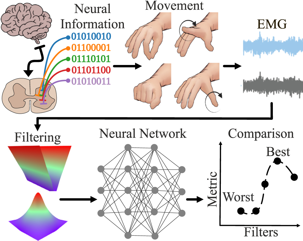
The signals necessary for precise finger movements originate in the brain and spinal cord. Alpha motor neurons in the spinal cord innervate the connected muscles, resulting in the production of movement (figure 1). The firing of a motor neuron produces a distinctive action potential, whose firing time can be simplified as a binary on and off state. Because a motor neuron fires multiple times during a movement, and there being multiple motor neurons involved, we refer to this as the binary code of movement. sEMG serves as a non-invasive method to record the summation of said action potentials by sensing the electrical activity that reaches the skin.

Figure 1. Precise finger movements are relayed from the brain to alpha motor neurons in the spinal cord. The temporal sequence of each action potential's firing can be represented as a binary series denoting on and off states. In this study, EMG signals were recorded from 13 subjects performing various movements. Frequency domain and spatial filters were applied to the signals. The number of signals was also reduced through ablations. An AI model was trained using the processed signals to analyze the impact of the filters on predicting hand kinematics.

Download figure:

Standard image High-resolution image

The sEMG signals however are prone to electrical and physiological noise [1, 2], which can be mitigated by filters in the spatial and temporal domains.

Given the absence of consensus regarding the optimal filters and electrode count required for accurate prediction of hand movements, here we aimed to assess and compare the efficacy of different temporal and spatial filters, alongside exploring ablation methods for electrode reduction. We conducted this investigation using an EMG dataset consisting of data from 13 subjects engaged in various hand movements (figure 2). We have recently developed a neural network that is capable of predicting the full kinematics of the human hand at multiple degrees of freedom [3, 4] with simultaneous and proportional real-time control [5]. Here, we aimed to investigate the impact of the pre-processing filters and ablation methods on the accuracy of the neural network in predicting hand movements based on the processed EMG signals. Due to the time-consuming nature of training a neural network, it is imperative to consider the potential effects of electrode count, spatial and temporal filtering. The frequency bandwidth of the sEMG is between approximately 10 and 500 Hz [1, 2, 6]. However, state-of-the-art myocontrol algorithms [7–11] rectify the signal and then apply low-pass filters below 5–20 Hz or compute the root mean squared (RMS) values from time intervals of 100–300 ms, which is comparable to said filters. Therefore, the main information used in conventional myocontrol applications is the low-frequency envelope of the signal that reflects the neural drive to the muscle responsible for motor execution. This information from the EMG is an estimate of the force exerted by the muscles. While this pre-processing is suitable to match the force frequency content, the sEMG may contain information relevant to the motor task that is not captured by the envelope [12].

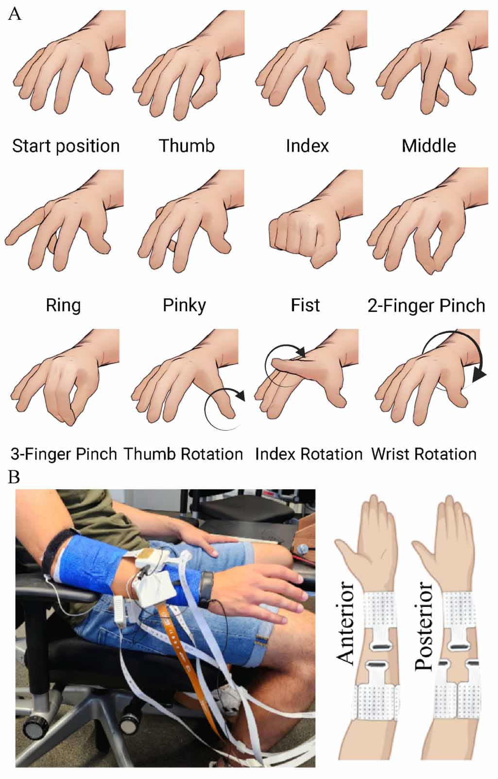
Figure 2. (A) All hand movements used in this study. The movements have been performed at two different speeds: 0.5 and 1.5 Hz. In depth description can be found in Sîmpetru et al [4]. (B) We used five electrode grids in our experiments. Three  s placed on the proximal part of the forearm and two  s above the wrist. The arm has been shaved and cleaned with an alcoholic solution prior to the electrode placement.

Download figure:

Standard image High-resolution image

In addition to temporal filtering, the sEMG can also be filtered in the spatial domain. Even a single physical monopolar electrode applies spatial filtering by integrating (averaging) the electric potential underneath the electrode. Moreover, linear combinations of monopolar signals are equivalent to the application of spatial transfer functions, which will depend on the distance between electrodes.

High-pass spatial filters have been used in sEMG recordings in order to increase the spatial selectivity over the recordings obtained with simple monopolar or bipolar systems [1, 13]. Such filters increase the recording selectivity, so that the contributions of motor units (MUs) far from the skin surface is reduced with respect to the sources in the vicinity of the electrodes [13, 14]. The higher the order of the filter, the lower the detected volume is. Spatial filters may be one-dimensional, such as the bipolar derivation, or two-dimensional (2D), such as the Laplacian [15–17].

Finally, the number of electrodes used for recording also influence the information content. Electrode grids with a larger number of electrodes are better for sEMG decomposition [1, 18, 19] but worse for real-time applications due to the high number of signals to process.

While we have a clear understanding of the intended effects and underlying principles of EMG filters, there is currently a lack of empirical evidence regarding the degree to which these filters preserve the information present in the unfiltered (Raw) EMG signal for estimating hand kinematics. In this work we attempt to answer this question by training the same model proven to work on unfiltered EMG [4, 5] following application of diverse temporal and spatial filters.

2.1. Dataset

We previously recorded data [3, 4] from 13 subjects (11 males, 2 females) during different hand movements (figure 2(A)) using 320 electrodes. The electrodes were distributed over three electrode grids (8 rows8 columns, 10 mm interelectrode distance; OT Bioelettronica, Turin, Italy) placed around the thickest part of the forearm and 2 around the wrist (13 rows5 columns, 8 mm interelectrode distance; OT Bioelettronica, Turin, Italy), proximal to the head of the ulna (figure 2(B)). Prior to the electrode grids placement, the skin was shaved and cleaned with an alcoholic solution. The monopolar sEMG signals were recorded using a multichannel amplifier (EMG-Quattrocento, A/D converted to 16 bits; OT Bioelettronica, Turin, Italy), amplified (×150) and band-pass filtered (0.7–500 Hz) at source, prior to offline analysis. The signals were sampled at 2048 Hz and collected using the software OT BioLab (OT Bioelettronica). While the sEMG signal was acquired, five pixel videos of the hand movement were recorded synchronously at 120 Hz by cameras (DFK-37BUX287, The Imaging Source™, Bremen, Germany) placed in different corners (upper/lower left/right) of a rectangular metal frame to capture multiple views of the same movement. The videos were processed by a custom trained neural network using the DeepLabCut [20] framework. A more detailed dataset explanation can be found in Sîmpetru et al [4].

Each movement was recorded for 40 s, resulting in a total data collection time of 12 min 40 s per subject. The recorded EMG data was saved as 2D matrices, with the two dimensions representing the 320 electrodes and the recorded time. For further processing, the EMG and kinematics data were divided into 93.75 ms windows with an overlap of 62.5 ms. The middle 20% of each movement's data is designated as the test set, while the remaining 80% is allocated for the training set. This results in 10 min 8 s training and 2 min 32 s testing data per subject. No validation split was used as our model was validated previously on the same data [3, 4] and on new one [5]. Additionally, in order to increase the amount of training data for our model, data augmentation was applied on each EMG segment. The augmentations used were Gaussian noise and magnitude warping [21] and offered a twofold training data increase, resulting in a per subject total of 30 min and 24 s.

The experiments were reviewed and approved on 8 March 2022, by the ethics committee of the Friedrich-Alexander University (application no. 21-150_3-B), ensuring compliance with the Declaration of Helsinki. Additionally, the subjects willingly signed an informed consent form.

2.2. Filters

We have evaluated a number of temporal and spatial domain filters, as well as a number of ablations in order to determine whether the prediction capability of the kinematics estimation model [3–5] will be affected.

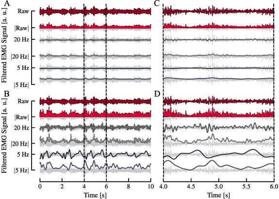
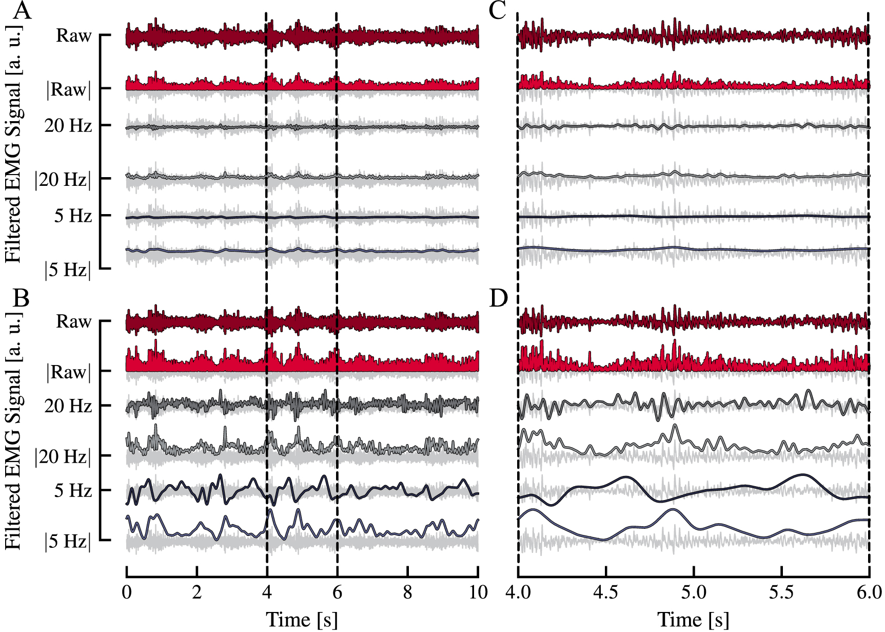
2.2.1. Temporal filters

For the temporal filtering (figure 3), we defined Raw as the unfiltered monopolar sEMG signals. From the Raw signals we derived two low-pass signals (5 Hz and 20 Hz) by filtering the sEMG segments backward and forward using a 4th order Butterworth filter with a cutoff frequency of 5 and 20 Hz respectively. These frequencies are the most common in the myocontrol literature because they are in the same frequency range that governs muscle force control [22]. Further, the rectified and low-pass filtered signals, specifically denoted as , , and , were obtained by first rectifying the raw EMG signal, and subsequently applying the filter. We also added the combination (denoted as Raw + 20 Hz) of the Raw and 20 Hz EMG signal, as we have previously found it to increase the accuracy of our model [3–5]. This combination can be seen as a temporal filter with the transfer function of  (s) where Hlow 20 (s) is the transfer function of the 20 Hz low-pass filter. We hypothesize that the higher accuracy obtained with this filter is due to the relative enhancement of the lower frequencies of the signal that contain information on the modulation of the firing rates of the active MUs [23].

Figure 3. Examples of the temporal filters used on an representative EMG signal. The signals in (A) were normalized to the 'Raw' signal, whereas the signals in (B) were normalized relative to their individual maximums, making the waveform differences easily distinguishable. (C) and (D) represent the zoomed-in time windows of the signals from (A) and (B) respectively. The nomenclature for the filters is as follows: 'Raw' represents the unfiltered EMG, while 'X Hz' represents the X Hz low-passed version of the EMG. 'Raw + 20 Hz' is not displayed as this is the combined input of unfiltered ('Raw') and 20 Hz low-passed ('20 Hz') EMG. Further the presence of denotes that the EMG has been rectified prior to filtering. The unfiltered EMG is depicted in a shade of gray to aid in understanding the effect of the applied filter.

Download figure:

Standard image High-resolution image

In total we evaluated the following temporal filters: Raw + 20 Hz, Raw, , 20 Hz, , 5 Hz, and .

2.2.2. Spatial filters

The spatial filters investigated in this paper include the longitudinal and transversal single and double differential filters (LSD, TSD, LDD, and TDD, respectively) [24], the normal double-differentiating filter (NDD), inverse binomial filter of order two (IB2) and inverse rectangle filter (IR) [24–26]. The spatially unfiltered signal can be seen as the signal filtered by the spatial identity operator (I). The masks corresponding to each of the applied filters are defined as follows:

2.2.3. Ablation

We also experimented with various electrode configurations commonly used in EMG studies. To do this, we manipulated the monopolar electrode signals by either removing or combining them in different ways. These alterations were referred to as 'ablations'. The ablations investigated in this paper include two large bipolar cases, one small single differential case and six other cases where electrode channels are randomly selected from each grid (figure 4).

Figure 4. Schematic overview of the ablations. The electrodes for the bipolars and single differential ablations have been chosen such that inter-electrode distance will be roughly equal. For the random monopolar electrode selection we select the electrodes in such a way that we achieve a uniform spread over the grid surface. The electrode grids are adapted from OT Bioelettronica's (Torino, Italy) official pinout manual.

Download figure:

Standard image High-resolution image

In the large bipolar ablation, for each electrode grid we took the two averages over a set of five neighboring channels each, placed either close to (forearm grid −20 mm apart; wrist grid −16 mm apart) or further away (forearm grid −50 mm apart; wrist grid −48 mm apart) from each other, and computed the difference between them. This mimics the effect of a bipolar measurement that uses electrodes with a large surface area [12]. In the single differential case, we selected two pairs of channels from each grid and computed the difference over the pair. Additionally, we took into account that the electrode grids used for the wrist have a different inter-electrode distance than those used for the forearm. Therefore, in both the large bipolar and small single differential case where the selected channels are meant to be further apart, we chose the measurements on the grid to be roughly at the same distance from each other for both the wrist and forearm grid.

In the remaining ablations, a random selection of channels across each grid was performed (5, 10, 20, 30, 40, and 50 channels). We ensured that once an electrode was picked, the probability of one of its neighbors to also be selected was lowered, which in turn increased the chance of electrodes from different areas of the grid to be chosen.

The number of input electrode channels for each ablation case is listed in table 2.

2.3. Model

We have utilized a previously published model architecture [3–5], which we have shown to be effective in decoding kinematics from EMG signals for both seen and unseen movements. This model has been implemented in Python using PyTorch (version 2.0.0+cu117) [27] and PyTorch-Lightning (version 1.9.4) [28]. While we will not go into detail on the model in this paper, readers can refer to the original source for more information. An architecture overview can be seen in figure 5 and a brief explanation of it will be provided as well as an in depth explanation on the model size reduction achieved for each filter.

Figure 5. Schematic overview of model architecture from Sîmpetru et al [5]. The EMG input is first reshaped and standardized. The first convolutional layer searches in the time dimension for motor unit action potential overlaps that are indicative of a specific movement phase. These overlaps get then compressed and integrated over the next convolutional layers so that the information not only within grids but also between grids is taken into account. The last part of the model is an multilayer perceptron that is used to map the high dimensional latent space into 3D coordinates. All the channel counts (C, , C1, and C2) can be seen in table 1.

Download figure:

Standard image High-resolution image 2.3.1. Architecture

The model's input is a 3D array, where the width represents time, the height represents the number of electrodes, and the depth corresponds to different frequency filters. Each frequency filter except for the Raw + 20 Hz filter contains information specific to a particular frequency range resulting in a depth size of 1. The Raw + 20 Hz filter combines the unfiltered data with the information filtered at 20 Hz using a low-pass filter and gives a depth of 2. The input is then reshaped and standardized grid-wise by subtracting the mean value and dividing by the standard deviation.

The deep learning model consists of two parts: a convolutional neural network (CNN) and a multilayer perceptron (MLP). The first convolutional layer looks for overlaps in the MU action potentials such that patterns can be found that are indicative of specific movements. These overlaps are then circular padded so the next layer can integrate not only inter-grid but also intra-grid information. The last CNN layer is used to further compress the information for the upcoming MLP. The CNN part of the deep learning model thus acts as a transform function that maps high frequency sEMG signals into low-frequency but high dimensional latent space. The second part of the model, the MLP, is used to map the high dimensional latent space produced by the CNN into 3D space.

2.3.2. Size

As can be seen in figure 5 the layer channel count is heavily influenced by the number of electrodes left after applying the spatial filter or ablation. Table 1 includes an overview over the channel counts for each spatial filter and ablation used. The input data can be described as a 3D array, where the depth represents the number of channels per electrode grid. The height of the array is made up of the electrodes of the forearm grids F and the wrist grids W. Spatial filters can be applied in the longitudinal, transversal or both directions and have an order of 1 or 2, depending on whether they are single or double differential (equation (1)). This, along with the number of rows and columns of the grids used, determines the number of reduced channels. Regarding the identity and ablation cases, the input array depth depends on the number of selected grid channels and can be mathematically expressed as follows:

where and refer to the order (single or double) of the longitudinal and transversal filter respectively. Since the channel count of the input can vary depending on the spatial filter or ablation used, the channel count of the hidden layers can also vary and is dependent on the input size. We denote these channel counts with C, CP, C1 and C2, each corresponding to a separate hidden layer as shown in figure 5.

Table 1. Channel counts per layer for each filter (see figure 5 for meaning). F and W represent the amount of channels remaining for the forearm and wrist grids respectively after applying a spatial filter or ablation. C is the channel count after reshaping and applying the first convolutional layer that operates only in time domain. After applying the circular padding we get . C1 and C2 are the channel counts after applying the last to convolutional layers.

FiltersModel parametersNameShort notation F W C C1 C2IdentityI646464963426Longitudinal single differentialLSD566060903224Transversal single differentialTSD565256843022Longitudinal double differentialLDD485555832921Transversal double differentialTDD483948722618Normal double differentialNDD363336542012Inverse binomial filterIB2363336542012Inverse rectangle filterIR363336542012Large bipolar close 111331Large bipolar far 111331Small single differential 2224415 random electrodes R555595110 random electrodes R10101010168120 random electrodes R202020203012430 random electrodes R3030303046181040 random electrodes R4040404060221450 random electrodes R50505050762820

They can be mathematically expressed as follows:

with their actual values being displayed in table 1.

2.3.3. Loss function

The loss function used was the mean absolute error. We chose this function because we wanted to linearly penalize any deviation from the ground truth.

2.3.4. Training setup

For the architecture chosen, we used the AdamW optimizer described in [29] with the AMSGrad correction from [30]. The weight decay was 0.32. We used the one cycle approach described in [31] as the learning rate scheduler with the upper bound being 10−2.5, the lower bound 10−7 and the initial learning rate 10−4. The models were trained for 25 epochs on 4 NVIDIA GeForce RTX 3080s with a batch size of 64 for each GPU. For this evaluation we used the same hyperparameter values as in Simpetru et al [4]. We choose 25 epochs as opposed to 50 or 75 as in previous works [3, 4] in order to make more efficient usage of our computing resources while still training the models sufficiently to reach a good level of accuracy.

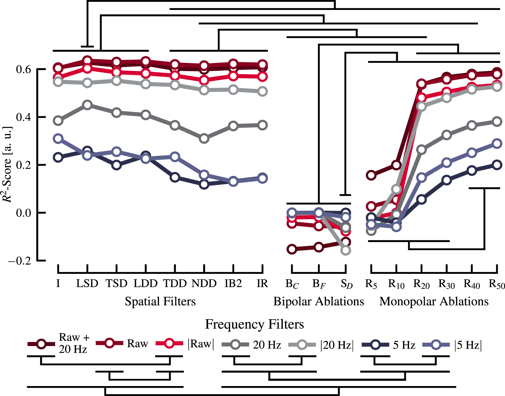
2.4. Statistical measures

To assess the significance of the observed differences among the different spatial and temporal filters (figure 6), two one-way analyses of variance (ANOVA) were performed for each filter type. A p-value lower than 0.05 was considered significant. Following the ANOVA, post-hoc t-tests with Bonferroni correction were conducted to further examine specific differences between pairs of group means. Again a p-value lower than 0.05 was considered significant.

Figure 6.  -score for different combinations of frequency domain filters with spatial filters and ablations. The nomenclature for the frequency filters is as follows: 'Raw' represents the unfiltered EMG, while 'X Hz' represents the X Hz low-passed version of the EMG. 'Raw + 20 Hz' represents the combined input of unfiltered and 20 Hz low-passed EMG. Further the presence of denotes that the EMG has been rectified. Both the spatial filters and ablations are denoted in their short form with the long name being described in table 2. Significance (p < 0.01) has been checked with post-hoc t-tests with Bonferroni correction.

Download figure:

Standard image High-resolution image

Table 2. Overview table showing the filter names, the results, and the number of electrodes used. From the results the -score is shown in figures 6 and 7(A). The training time is shown in figure 7(D). The best results are denoted in bold and slightly bigger font.

FiltersResultsNumber of electrodesNameShort notation -scoreCorrelationEuclideanTrainingForearm gridWrist gridTotal(a.u.)Coefficient (a.u.)Distance (mm)Time (min)IdentityI0.610.835.7722.556464320Longitudinal single differentialLSD 0.63 0.84 5.58 20.455660288