Our focus is on haemophilia A, a blood clotting disorder where a deficiency of FVIII results in elevated (spontaneous) bleeding risk. Haemophilia A patients are treated by intravenous injection of FVIII at regular intervals. The PK of FVIII is often described using a two-compartmental structure, where the first compartment represents the distribution of FVIII into the blood and the second is often thought to represent the initial rapid clearance of FVIII or its binding to intra or extra-vascular space [12,13,14]. The two-compartmental model can be represented by the following system of partial differential equations:

$$\beginc} }}} =& }} + A_ \cdot k_ - A_ \left( + k_ } \right)} \\ }}} =& \cdot k_ - A_ \cdot k_ } \\ \end$$

(1)

Here, the rate constants \(k\) describe the flow between the compartments specified in its subscript, \(_\) represents the concentration in the 1st compartment (and so on), and \(I\) represents the rate of drug entering the first compartment after drug administration. The rate constants \(k\) are functions of the PK parameters: \(_=\frac_}\), \(_=\frac_}\), and \(_=\frac_}\) with \(z=\_,_\}\) referring to clearance, inter-compartmental clearance, central distribution volume, and peripheral distribution volume, respectively.

Consider a population of \(n\) individuals with \(\mathcal=^,^,^\right)}_\), each with irregular drug concentration measurements \(y^ \in }_^\) sampled over time horizon \(^\in \left[0,_\right]\) with \(_\) indicating the follow-up time for individual \(i\). Drug concentration predictions are produced based on the compartment model and a matrix of interventions \(^\) containing information on time of dose, dosage, and infusion rates that affect the integrator at the specified time points:

$$\hat^(t) = A\left( ,I^ } \right)$$

(2)

In non-linear mixed effects models, individual estimates of each of the PK parameters \(z^ \in }_^\) are obtained based on covariates \(^\in }^\) and subject-specific random effects \(^\sim N\left(0,\Omega \right)\), where \(\Omega\) is a \(M\times M\) covariance matrix when random effects are included on all PK parameters. The following implementation is frequently observed within the pharmacometrics literature:

$$z_^ = \theta_ \cdot \exp \left( ^ } \right) \cdot \mathop \prod \limits_^ }} f_ \left( ;\theta_ } \right)$$

(3)

Here, \(\theta\) represent model fixed effect parameters and \(_\subset \left[1..D\right]\) indicates the subset of covariates used to predict \(_\). After specifying a model for the residual error \(\epsilon \sim N\left(0,\Sigma \right)\) on \(^\) (e.g. additive, proportional, or a combination of both), model parameters \(\Theta =\\) can be optimized by maximizing:

$$\hat = \arg \max_ }\left( \Theta \right) = \mathop \prod \limits_^ p\left( |\Theta ,\eta^ } \right)p\left( } \right)$$

(4)

As previously mentioned, development of non-linear mixed effects models requires considerable time and expertise, partly due to the manual selection of covariates and the functions \(f\) to represent their effect on \(z\). In DCMs, the fixed effect model is learned by a neural network \(\phi\) with parameters \(w\), and the covariates are used to predict typical PK parameters \(^\):

$$\zeta^ = \phi \left( ;w} \right)$$

(5)

And the model minimizes the squared error:

$$\hat = \arg \min_ }\left( w \right) = \mathop \sum \limits_^ \mathop \sum \limits_^ }} \left( ^ - A\left( ^ ;\zeta^ ,I^ } \right)} \right)^$$

(6)

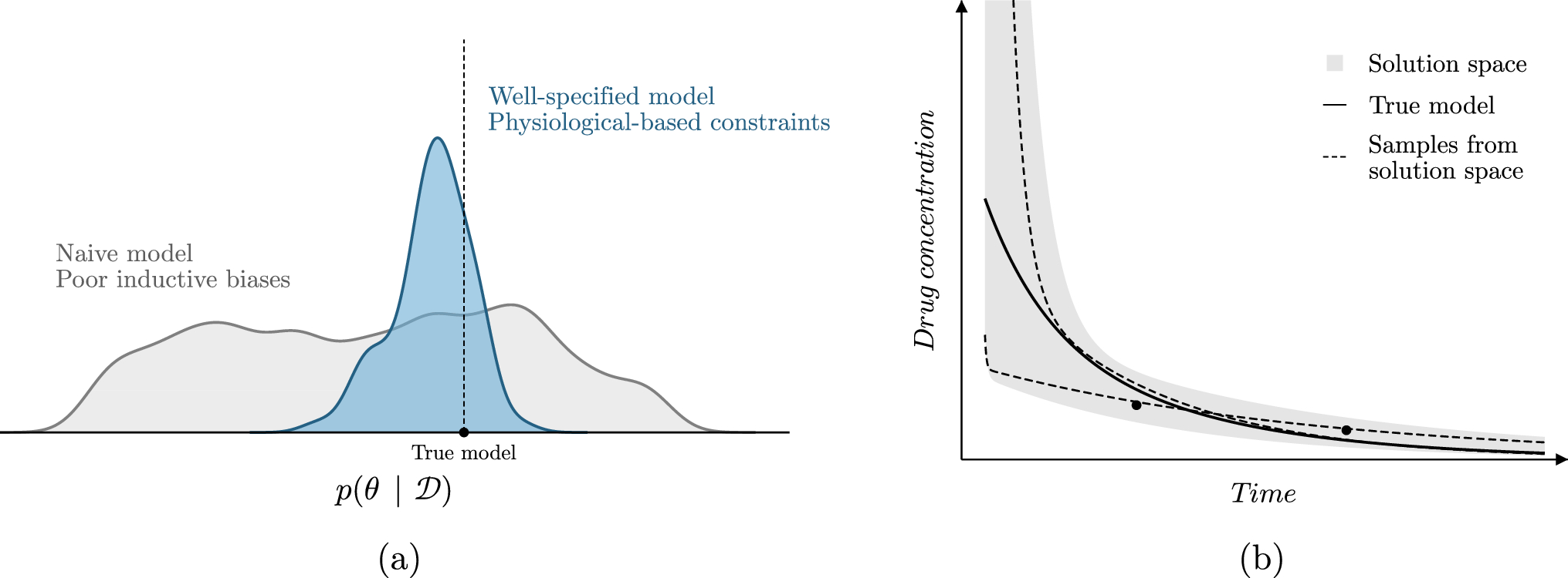
These models are relatively unconstrained in their prediction of \(^\), as long as it results in low error with respect to the observations. It can thus be the case that the model is not penalized for making extreme predictions outside of the observed data.Model constraints.

We propose three simple approaches for constraining the solution space of DCMs (Fig. 2). First, boundary conditions were imposed on the PK parameters by using a transformed sigmoidal function following the output layer of the neural network (referenced as boundary constraint; Fig. 2b). The boundaries can be set empirically based on prior knowledge. For example, bounds for the volume of distribution of drugs tightly bound to plasma proteins can be based on the expectation that the plasma volume of a typical male is roughly around 46—52 mL/kg [15]. Lower bounds of [0, 0.3, 0.05, 0] and upper bounds of [0.5, 7, 0.5, 2] for respectively \(CL\) (L/h), \(_\) (L), \(Q\) (L/h), and \(_\) (L) were used.

Graphical models representing the model structure of the proposed architectures. Naive (a), boundary constraint (b), global parameter (c), and multi-branch network (d) architectures are depicted. Nodes represents neurons, with the coloured box representing the hidden layer of the neural network

Next, global parameters \(\theta\) for a subset of the PK parameters were estimated in parallel to \(w\) (referenced as global parameters constraint; Fig. 2c). We chose to estimate \(\theta =\_\}\) since these parameters affect the early distribution of FVIII, and drug concentration measurements at early time points are usually too sparse to identify covariate effects on these parameters.

Finally, we describe a neural network architecture where each covariate (or specific combinations thereof) are connected to specific PK parameters via independent sub-models, whose predictions are combined using a product (referenced as the multi-branch network; Fig. 2d). This architecture is similar to a generalized additive model, using product accumulation rather than the sum of covariate effects. The use of a product matches the standard implementation of covariates in population PK models (Eq. 3), and facilitates the interpretation of the clinical relevance of each covariate. For example, covariates resulting in a maximal net change 20% of the corresponding PK parameter are often deemed clinically insignificant in the pharmacometrics literature [16]. An additional benefit of the approach is that the output of each sub-model can be visualized, allowing for the interpretation of the learned covariate effects. A schematic overview of the multi-branch network is provided in Supplementary Fig. 1.

More details about the specific implementation of the model constraints can be found in Supplementary Data 1A.

We simulated a data set of haemophilia A patients based on population data from the American National Health and Nutrition Examination Survey (NHANES) [17]. The weight, height, and age of 756 male individuals without missing data were collected from the data set and used as covariates. FVIII levels were simulated based on an existing population PK model of an extended half-life FVIII concentrate [18]. This model was chosen as it used an estimate of the fat-free mass (FFM) from [19] to predict FVIII clearance (\(CL\)) and central volume of distribution (\(_\)):

$$FFM = \left( }^ }}} \right) \cdot \left( \right)}}} \right)$$

(7)

This allowed for the comparison of model accuracy when training models using FFM directly as well as using its components weight, height (as part of BMI), and age. This could give an indication of the accuracy at which non-linear interactions of covariates could be learned.

The previous PK model was based on a two-compartment model, with inter-individual variability on the \(CL\) and \(_\) parameters. Using the structural equations reported by [18], typical estimates of the PK parameters were produced. Next, samples of the random effects were drawn to produce individual estimates of the PK parameters. Each individual received a dose of 50 IU/kg, rounded to the nearest 250 IU. To allow for stochasticity of measurement times, samples were taken from a multivariate normal distribution \(^\sim N\left(\left[\mathrm\right],\sigma =\left[\mathrm,5\right]\right)\). Sampling times were truncated at \(t=0.25\) (i.e. 15 min after dose) to prevent samples at negative time points or too close to the time of dose administration. Finally, the ODE was solved based on the individual PK parameters to simulate FVIII levels for each individual and additive error (\(\sigma =5.0\) IU/dL) was added to create the training data.

Prediction accuracy of the proposed constraints was compared to a naive neural network as well as the initialization approach suggested in [9]. In all experiments, covariates were scaled between 0 and 1 using min–max scaling. Models were trained using patient weight, height and age, or FFM and age. A two compartment model was used. Each neural network was trained using a single hidden layer of either 8, 32, or 128 neurons followed by the swish activation function [20]. A softplus activation function was used in the output layer of the naive neural network as well as in the model estimating global parameters for \(Q\) and \(_\) to constrain latent variables to \(}^\). All models were trained for 500 epochs using the ADAM optimizer with a learning rate of 1e-2 [21]. We found that these settings were sufficient for each model to converge before the end of optimization. First, prediction accuracy and robustness of the naive, initialization, boundary, and global parameter models were compared. The multi-branch network was not tested in this context due to similarities to the global parameter model. Each model was fit to a random subset of the simulated data of size 20, 60, or 120 to represent data sets of small, medium, and large size, respectively. A Monte Carlo cross validation of 20 different train and test sets was performed in order to estimate the stability of model predictions. In addition, model training was replicated five times on each train-test split. This resulted in a total number of 100 replicates of each model, which was deemed sufficient to estimate model variability given our computational budget. Model accuracy was represented by the root mean squared error (RMSE) of predicted FVIII levels compared to the true, simulated concentration–time curves on the test set. To this end, true and predicted FVIII levels were collected at five minute intervals until \(t=72h\) as a means to approximate the error compared to the full concentration–time curve. Models were compared in terms of their median RMSE over the 20 data sets and five model replicates. Model robustness for each of the architectures was represented by the percentage of models with RMSE greater than 150% of the median RMSE (references as divergent models).

In order to evaluate differences between using fully-connected versus multi-branch neural networks, the data set was augmented with two continuous and one categorical covariate without correlations to the other covariates. For the continuous covariates, random samples were drawn from Uniform(0,1) distributions, while for the categorical covariate samples were randomly assigned to one of five categories with equal probability. Next, three models with global \(Q\) and \(_\) parameters were fit to FFM, age, and the noise covariates: (1) a fully-connected model, (2) a multi-branch network with all covariates independently connected to \(CL\) and \(_\), and (3) a multi-branch network with the ground truth covariate connections as used in the simulation (referenced as the causal model). Fully-connected models were trained using a single hidden layer of 32 neurons. The number of neurons in the hidden layer of each sub-model was set to 16 to ensure that models had roughly similar number of parameters. Accuracy was again compared using the RMSE. Results were compared with the global parameter models trained on FFM and age from the first experiment (models trained using 32 neurons). Covariate effects from the multi-branch network were visualized to facilitate model interpretation (See Supplementary Data 2 for implementation details).

All model code and synthetic data will be made available at https://github.com/Janssena/dcm-constrained.

We compared the predictive performance of two previously published population PK models [22, 23] to the DCM with or without the proposed constraints and a Neural-ODE based model [8]. Data consisted of 69 severe haemophilia A patients who received a single dose of 25–50 IU/kg standard half-life FVIII. For each patient, three measurements were available roughly 4, 24, and 48 h after dose. Available covariates without missing data were patient weight, height, age, and blood group.

The population PK model by [14] included the effect of weight on all PK parameters, as well as the effect of age on \(CL\). The model implemented allometric scaling, which is very common in PK models. We also evaluated the performance of a more recent model by [23]. Instead of using weight, this model implements the effect of FFM on clearance and volume of distribution. An effect of patient age was also included on clearance. Since it is well documented that patients with blood group O have higher FVIII \(CL\) compared to non-O patients, we also fitted models including a proportional effect of having blood group O on \(CL\) [24].

DCMs were fit using neural networks with a single layer containing 8, 32 or 128 neurons (halved for each sub-model for the multi-branch network). For the fully-connected network, model input was patient weight, height, age, and BGO. Models were fit without constraints, using boundary constraints (same as used during simulation experiments), and using global parameters for \(Q\) and \(_\). In the multi-branch network clearance was predicted based on patient a combination of weight and height, age, and BGO, while estimating volume of distribution based on a combination of weight and height. Global parameters were estimated for \(Q\) and \(_\) in all models.

For the Neural-ODE based model we followed the general architecture by Lu et al. [8]. Hyper-parameters were the number of neurons in the encoder, Neural-ODE, and decoder (8, or 32), the number of hidden layers (1 or 2) in the Neural-ODE, and the number of the latent variables (2 or 6). Encoder and decoder consisted of a single hidden layer. Tanh activation functions were used in the Neural-ODE to improve model stability. Model input was patient weight, height, age, and BGO and values were normalized between − 1 and 1. This marks an important difference to the model by Lu et al., where part of the drug concentration measurements were used as input to the encoder and decoder.

A ten-fold cross-validation was performed for both the non-linear mixed effects models and DCMs. Both PK models were implemented in the NONMEM software (ICON Development Solutions, Ellicott City, MD) and model parameters were re-estimated on each full train fold. Exponents of the effects of weight on the PK parameters were not re-estimated in the model by [14] since they follow the concept of allometric scaling. The accuracy of typical predictions were reported. The ML models were trained for 4000 epochs which was more than sufficient for model convergence, and neural network weights resulting in the lowest validation error (20% of training fold) were saved. Hyper-parameter selection was performed by comparison of the RMSE on the validation sets. Results for the models with lowest average validation error were presented. The average RMSE of predictions with respect to the test fold was reported.