In the raw data (figure 2(Ci)) there is a clear anisotropy, with near neighbors more likely to be found on the sides than the front or back. This, however, might be an artifact of the animal's body shape; locusts are not circular but have an elliptical body shape. Elongated shape allows nematic ordering which could be evolutionarily adaptive for collective movement. Due to the elongated, ellipsoid shape (see figure 7(A)) of locusts, the body centers of locusts at the side are closer than at the front or back. This effect increases with the packing fraction, as in tightly packed groups the nearest neighbor distances of body centers decrease and are increasingly affected by minimal distances imposed by their body shapes [38–40]. At lower packing fractions, locusts tend to be more loosely assembled, and the body shapes have less influence on the alignment of the locusts.

We can correct for this bias by rescaling the raw coordinates with the aim being to take the elliptical body shapes and transform them to circles. In this data set the alignment is high, since the locusts are all marching in the same direction through a channel, so the velocity vectors (and hence the orientations) of all individuals lie along roughly the same direction. Because of this alignment we can apply the same transformation to all individuals with approximately the same result. Since we have rotated our data so that the mean velocities are always along a principle direction we can perform this rescaling operation by multiplying the coordinates along one principle direction by a scale factor. The scale factor was derived from the aspect ratio of the bounding boxes obtained from tracking and determined separately per video, in total 0.54 ± 0.06. We then used this scale factor to correct the shape by squeezing the long x-axis to obtain a 1:1 ratio. This data is referred to as 'rescaled' and an example of the result of this process is shown in figures 1(C) and (D). The nearest neighbor distribution over the rescaled data is roughly uniform (figure 2(Cii)), indicating that there is no preference for side to side distribution (figure 2(B)). The observed difference in the unscaled data is due to body-shape anisotropy [38]. The effect of rescaling is consistent across all recordings (figure 2(A)).

Since the distribution of neighbors (in the corrected coordinates) is radially symmetric we can use the radial distribution of neighbors as a way of quantifying the physical structure of the group. The RDF is a common way of quantifying the local structure of materials and small molecules. The RDF measures the local density of neighbors relative to a focal particle (or in our case individual), averaged over all particles, as a function of radius. On a perfectly ordered lattice the RDF will display sharp peaks at distances corresponding to the locations of neighbors. The shape of the RDF provides qualitative information about the state of a material system. For example, as a system heats up, the particles oscillate about their equilibrium positions and the sharp peaks in the RDF which would be observed for static particles become more diffuse [41]. More diffuse peaks indicate higher disorder.

For our data we calculate the RDF as a way of qualitatively comparing the distribution of marching locusts to the expected RDF for various states of matter to understand what physical state the marching locusts most resemble. The RDF is calculated as

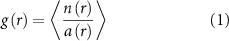
where n(r) is the number of individuals in an annulus of radius r relative to a focal individual, a(r) is the area of this annulus (thus is the density of individuals in the annulus of radius r) and the brackets denote the average over all individuals. This is computed for specific regions in two of the recordings where we expect densities to be the highest (videos 1 and 2). In low density videos there is too little data (too few individuals for too short a recording) for the function to converge to a steady shape. We focus on regions which are in rectangular strips above and below the obstacle and in the 'funnel' region of the frame (see the definitions in section 2.1.2). In these regions the densities are high but the channels are narrow so the number of individuals and their neighbors is somewhat low. Further, many individuals are close to edges, which if not properly accounted for strongly skews the RDF. To deal with this we consider the boundaries of the selected region to be periodic. With this consideration we eliminate the effect of the edges without losing the contributions of the individuals that lie near an edge. These calculation are all performed on the rescaled data.

The placement of the elongated obstacle varies across the two recordings. In video 1 the channel is nearly symmetric with the elongated obstacle placed in the center. In video 2 the elongated obstacle is placed asymmetrically, closer to one side of the channel. Because of this placement there is a wide channel and a narrow channel. We only include the wide channels in calculating the RDF for this recording. For the nearly symmetric recording we calculate the RDF in both channels (labeled 'top' and 'bottom' in figure 3(B). The calculated RDFs are shown in figure 3. There is a clear first peak at a distance of roughly 5–6 cm sometimes followed by a weak second peak at roughly 10 cm. This second peak only appears in the highest densities and indicates some qualitative similarity to a liquid crystal [42] especially as compared to random packed hard spheres [43] for instance. The presence of some amount of order in the RDF lends support to our consideration of this system as fluid-like.

Figure 3. (A) A cartoon of the radial distribution function for Lennard–Jones disks in the solid, liquid, and gas phases. (B) The radial distribution functions for the highest density regions in videos 1 and 2. The dashed line is , which the RDF should converge to at long distances.

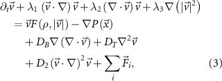
Download figure:

The main aim of this paper is to evaluate the validity of a macroscopic description of marching locusts and the corresponding macroscopic variables. In this section, starting from a general hydrodynamic description, the Toner–Tu equation, we argue that in the continuous limit a simple relation between pressure and density holds:

We tested this relationship by computing the hydrodynammic pressure using the tracked and rescaled locust data in a one-dimensional approximation and under steady flows. Notably, this linear dependence is similar to ideal gas-like behavior. A similar resemblance to ideal gas has been observed in human crowd dynamics (see, for example, [44]). Additionally, a non-linear generalized ideal gas law has been used to describe the thermodynamics of swarming midges [45, 46]. It suggests that the thermal equilibrium may be a good approximation in those regimes. In this case the equation of state may provide predictive power for a wide range of densities and boundary conditions. A priori we do not expect to find that an equation of state holds for active fluids. We usually find equations of state in thermal equilibrium and the current system is far from it. In addition, the general functional form of the pressure is unknown, but using our data we can find its approximate dependence on the density. Some recent studies of an equation of state for active matter and systems far from equilibrium include simple models of active particles and active colloids [47–54] and only a few examples for biological systems [44–46]. In [7] a minimal version of the Toner–Tu equations was studied and the same equation of state was assumed (equation (2)). There it is described as an adjustment of the velocity intended to flatten the density field by creating a force towards homogeneity since the pressure term then 'punishes' gradients in density (see equation (3)).

In addition, this equation of state (equation (2)) for the hydrodynamic pressure motivated us to look at the mechanical pressure, which is related to deformations and not to the kinetics of the fluid. In thermal equilibrium they are balanced and equal. Therefore, we do not expect them to be equal when the system is far from thermal equilibrium (see also [55]), as in the current active system, which is studied here. Nevertheless, we find a similar linear relationship between the pressure and density for a similar range of densities.

The Toner–Tu equations [56, 57] can be written in the following schematic form:

where are coefficients of advection/convection-like terms. This is the most general form of such terms. Under the requirement of Galilean invariance, which means that the laws of motion are the same in all inertial frames of reference, the equation is reduced to the Navier–Stokes equation when . The additional advective terms that are allowed by the lack of Galilean invariance (when or ) may represent behavioral responses to gradients of velocity components in various directions. is an effective restoring force that keeps the speed constant at v0. This preferred speed breaks Galilean invariance by defining a preferred reference frame. In principle can be any one-dimensional function so that , but in order to create the spontaneous breaking of symmetry at a critical density ρc towards a particular direction of movement this function can be of the form

where α and β are positive constants and

(see [7, 58] for more details). The speed relaxes in the time to v0 and thus in the hydrodynamic limit this term does not contribute. Moreover, we will consider only averages over long times when the system reaches stationary state and the individuals are highly aligned (times much greater than the relaxation time). is the hydrodynamic pressure whose gradient is the total acceleration of the fluid particles (the local and the convective accelerations). This pressure is identified as the trace of the bulk stress tensor, whose microscopic definition is in terms of momentum fluxes [59]. As mentioned above, for active matter this definition does not coincide in general with the mechanical pressure that is described below [55]. are coefficients of the viscosity-like terms. They contain the second order derivatives with respect to the spatial coordinates and are thus important when there are rapid spatial variations. In our case, they are small relative to the convective terms (which are first order in the derivatives) since we concentrate on slow spatial variations in the long wavelength approximation. We will see that in our approximation and therefore , which justifies the hierarchy of the derivative expansion. The s are all of the additional external forces that may act on the fluid.

Another work [7] suggests that a similar equation of state (equation (2)) can come from looking at the expansion of the pressure in the following form that was introduced by Toner and Tu [56]:

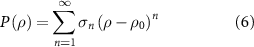
where ρ0 is the mean density. If we keep only the leading order of this expansion we get a pressure term that keeps the density of the fluid close to the mean value. Plugging it in equation (3) we are left only with the density gradient.

The locusts are funneled into a narrow region split into two channels by an elongated obstacle, shown in figure 4(A). The obstacle induces an increase in density and a corresponding decrease in speed (figures 4(D) and (F)). The presence of this funnel and obstacle creates variations in the density and velocity from left to right across each frame. We choose to divide the video into two regions, one above and one below the obstacle, indicated by the white rectangles in figure 4(A). In addition to this spatial division, for each region we seek time windows in which both the average density and average velocity are approximately constant, consistent with a continuity equation:

Figure 4. (A) A snapshot of video 1 with the areas used for analysis marked by white boxes. All panels show analysis of quantities averaged over time for the bottom strip. (B) The horizontal component of the velocity vx as a function of the horizontal coordinate x (average over time).(C) The ratio of the velocity components squared as a function of x. (D) The density (packing fraction) as a function of the horizontal coordinate x. (E) The alignment order parameter as a function of x. The thick horizontal blue line denotes the segment where the alignment is maximal . (F) The horizontal component of the velocity vx squared as a function of x.

Download figure:

We consider the system in a time segment to be in a steady flow if the standard deviation of the velocity and density are less than 10 percent of their mean value. We show in the SI how they are satisfied for long periods of time in the two strips of video 1 (330 s approximately for the bottom strip and 120 s for the top strip). In the following analysis we use these steady regions to compare the dynamics of the locust movement in the continuum limit with the Toner-Tu equations.

In this section we only consider time segments when our steady flow conditions are satisfied. The experimental arrangement in the field created an effective two-dimensional funnel that focuses the marching locusts towards the elongated obstacle (the bottle in the recording or the funnel region), around which the density is increased and the speed is reduced relative to the other regions. After passing the obstacle the locusts spread out, lowering their density but increasing their speed. Note that every point in the plots of figure 4 is obtained by averaging over a long time period in which the strip is in steady state.

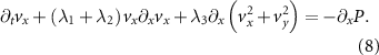
The funneling effect of this geometrical structure makes it attractive to consider a one-dimensional approximation for the dynamics of the system. This allows us to consider mean values of the variables along narrow vertical strips at constant x and to neglect their variation with respect to the vertical coordinate y. Within this approximation, the alignment force is small relative to the convective acceleration, and the Toner–Tu equation (3) are reduced to the following:

To compute time averages the data is binned into strips 50 pixels wide in the x dimension which is roughly 4 cm, or the average length of a locust. In figures 4(B) and (D) we see the density and the horizontal component of the velocity vx as a function of the horizontal distance, x, where the angle brackets denote average over time.

The ratio as a function of the position on the horizontal axis (x direction) is less than 0.1 (figure 4(C)) indicating that the term is small relative to the x component, thus this term can be neglected and we obtain the following equation:

where

In addition, we find that in steady flow the local acceleration is negligible compared to the convective one. That is an additional simplification of equation (9). We can see this by taking the average over time of equation (9). From the integration of the first term of the left-hand side over a time segment T we get the mean acceleration which is bounded by a small number for a long time of measurement ( s, see figure S2B-D in the SI)

compared to the second term where and  (cm s−1)2. In conclusion, we see from the data that in the one-dimensional approximation the convective acceleration is the dominant term in its contribution to the total acceleration.

Assuming that the linear dependence of the pressure on the density in equation (2) is correct and that the one-dimensional approximation is good enough, we get from equation (9) that the density should be linear with the velocity squared:

The Toner–Tu equation gives us a possible interpretation of this linear relation as Bernoulli's principle—the higher the speed of the fluid, the lower the pressure that it exerts, and the weaker force that this pressure produces works towards stabilization of inhomogeneities in the density (see [7] and the discussion after equation (2)). However, the accuracy of this relation (12) depends mainly on the accuracy of the one-dimensional approximation of the hydrodynamic equations. When all individuals are aligned along one principle axis, this linear relation should be valid. To check this we can quantify the alignment by introducing an alignment order parameter [3]

where χ is the angle between the local velocity and the average direction of movement (see figure 4(A). The overline denotes the average over all individuals. Q = 0 is when all the particles are in random orientation and Q = 1 when they are perfectly aligned. It was observed in [60] that individual locusts tend to move more randomly in groups with low alignment. This noisy motion appears to help locust groups to reach the highly aligned state. From the Toner–Tu equation (3), we expect that when the alignment is strong, the one-dimensional approximation is reasonable and the linear relation (12) should hold. The average alignment in steady flow is given in figure 4(E) and in figures 4(D)–(F) the segments where the alignment is strongest are denoted by a thick horizontal blue line. In the bottom strip the alignment is maximal () for  cm (marked by thick horizontal blue lines in figure 4(E)), and for  cm in the top strip (the details about the top strip appear in SI). For those segments we then check the linear correlation of with and find that it is stronger in the segments where the alignment is stronger (figure 5 ). We see that indeed the linear fit is significantly better when only the region of strong alignment is included, supporting the validity of equation (2) in the one-dimensional approximation. In general, we expect that the equation of state holds everywhere where the pressure is sufficiently high.

Figure 5.  as a function of - for the bottom strip (the mean velocity squared vs. the negative mean density). The red points correspond to regions of strong alignment (from figure 4) and the yellow points include all regions, regardless of alignment. The linear fit of the points with strong alignment is in red and . When we include all the points in the fit we get the dashed yellow line with .

Download figure:

We tested the same linear relation over more recordings but they are, as evident in figure S6 in the SI, at densities which are too low to contain a sufficient number of animals for analysis, and have low polarization as well (maximal mean value of 0.8). The results for the top strip of video 1 are given in the SI (figures S3, S4). In the second recording the top strip is too narrow for a significant stream. In figure 6 we summarize values of the velocity squared vs. density for three segments of strips with highest alignment (Q > 0.95) and obtain strong linear fits.

Figure 6.  as a function of - for segments of strong alignment () with linear fits (the mean velocity squared vs. the negative mean density). The red points correspond to the top strip of video 1 (), the yellow points for the bottom strip () and the purple points are for the bottom strip of video 2 ().

Download figure:

In the previous section we developed a hydrodynamic definition of the pressure, which is proportional to the squared velocity. Additionally, we can define a static pressure through an analogy with the mechanical stress. The mechanical stress is defined as the force per unit area acting on the surface of an object and is related to the strain (or deformation of that object) by a generalized version of Hooke's Law [61]. In the context of marching locusts we can think of the object as the area which an individual locust occupies and can calculate the force that must be exerted to shrink or grow that area relative to a fixed reference size. We approximate the area occupied by a locust as the Voronoi area around the individual. Because the distribution of neighbors in the corrected coordinates is radially symmetric we approximate the area around an individual as circular. This ensures that the mechanical pressure is radially isotropic and one-dimensional. Thus we define our mechanical pressure, , proportional to the isotropic strain of this circular area, which we can write

where r is the radius of the circle representing the area occupied by a single locust and is the change in the radius relative to the reference radius, rm . To calculate the area occupied by a single locust we start by computing the Voronoi tessellation of a single frame, including the positions of all locusts, except for those on the edges. The area around a given locust is taken as the area of the corresponding Voronoi cell. The radius of the circle, r, with the same area as the Voronoi cell is computed for each individual. This process is illustrated in figure 7. In what follows we calculate the reference radius, rm, per frame as the mean radius taken over all locusts in that frame.

Figure 7. An illustration of the process for determining the radii, r, used in calculating the mechanical pressure. (A) A snapshot of the locusts with the tracked centroids overlaid. The image is stretched to match with the centroids in the rescaled coordinates. (B) The Voronoi tessellation over the points of the snapshot in (A). (C) The circles that were generated from this tessellation. Each circle in (C) has an area equal to the corresponding Voronoi cell area shown in (B).

Download figure:

In addition to the pressure we calculate the local packing fraction around each locust,

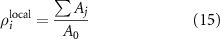
where the summation is over all neighbors within a fixed radius, r0, of a focal individual, Aj is the area of the bounding box of a single neighboring locust and A0 is the area of the circle with radius r0. We choose r0 to be roughly nine locust body lengths (36 cm) and from this calculate the number of locusts in the that circle. This is because the maximum value of the local density distribution is roughly constant for r0 values above six body lengths (24 cm) but drops off, due to edge effects, for values higher than 12 body lengths (48 cm). Thus we choose a value between these bounds and from this calculate the number of locusts in that circle. The mechanical pressure vs packing fraction is shown in figure 8. There is, as with the hydrodynamic pressure, a strong linear relationship between the mechanical pressure and the local density. In general there is not always a well defined pressure in active systems [55, 62]. Here we find a consistent linear relationship between two definitions of pressure with the density, indicating that despite the active nature of this system the pressure can be a well defined state function for a range of densities.

Figure 8. The mechanical pressure (equation (14)) vs local packing fraction (equation (15)) for two recordings which span a large range of densities (video 1 and video 2). The points are the mean values of all points in fixed size bins (all containing the same number of samples) and the spread of the bands is the first standard deviation. The black lines are linear regressions on the displayed regions of each recording. The R2 values for videos 1 and 2 are 0.982 and 0.999 respectively. The dotted line is the line where the mechanical pressure is 0. Note that the mechanical pressure here is defined dimensionless (without an 'elastic constant') and is relative to the mean radius in a given frame.

Download figure: