Study design

A total of 213 women in their 3rd trimester enrolled in the larger MADRES cohort were recruited into this personal monitoring sub-study between October 2016 and March 2020. MADRES is an ongoing prospective pregnancy cohort focused on predominantly low-income, Hispanic women and their babies residing in Los Angeles, CA. MADRES aims to address critical gaps in understanding environmental health disparities and the impacts of air pollution and social stressors on maternal and child health. The details of eligibility, enrollment, and follow-up of participants are described elsewhere [36]. Briefly, eligible participants for this sub-study were in the 3rd trimester at the time of recruitment, ≥18 years of age, and could speak either English or Spanish fluently. In the initial design, people living in a household with an active smoker were excluded to reduce the impact from smoking on personal PM2.5 exposures. However, in order to encourage all participants to contribute to sub studies, the non-smoking household criterion was not applied consistently throughout the study and was eliminated by the end of 2018. Informed consent was obtained for each participant. The University of Southern California’s Institutional Review Board (IRB) approved the study protocol.

Data collection

The 48-hr integrated personal PM2.5 measurements were collected to characterize the composition of personal PM2.5 and identify its main sources in the MADRES cohort through source apportionment analysis. Several other data sources were used from MADRES questionnaires and measurements and from external data sources in a second follow-on bivariate analysis to confirm source identities and understand the personal drivers that affect the mass contribution of each source. These included the following: questionnaires (collected at trimester 1, 2, and 3, respectively), GPS-derived time-activity patterns and environmental exposures within activity spaces from the personal monitoring study, modeled residential environmental exposures, and outdoor EPA PM2.5 chemical speciation data from a central site.

Personal PM2.5 measurements

The personal PM2.5 sampling design and protocol in the 3rd trimester is described in detail in O’Sharkey et al. [37] and Xu et al. [38]. Briefly, personal, 48-h integrated PM2.5 measurements were collected using a Gilian Plus Datalogging Pump (Sensidyne, Inc.) operating on a 50% cycle at 1.8 lpm flow rate with the sampling inlet located in the breathing zone. The pump is connected to a PM2.5 Harvard Personal Environmental Monitor (PEM) size-selective impactor with a 37 mm Teflon filter (2 µm pore size; Pall, Inc.). Participants were asked to wear the sampling device for the entire data collection period with a few exceptions. These included when it is unsafe to do so (e.g., driving), showering, or sleeping, in which case they were instructed to place the device near them in an unobstructed location.

Filters were analyzed gravimetrically to determine PM2.5 mass using an MT5 microbalance (Mettler Toledo, Columbus, OH, USA) in a dedicated humidity- and temperature-controlled chamber at the USC Exposure Analytics Laboratory. Filters were then sent to RTI International (Research Triangle Park, NC) to determine elemental composition of the following 33 species using Energy Dispersive X-Ray Fluorescence (EDXRF): barium (Ba), calcium (Ca), chlorine (Cl), copper (Cu), iron (Fe), potassium (K), magnesium (Mg), manganese (Mn), sodium (Na), nickel (Ni), sulfur (S), silicon (Si), titanium (Ti), zinc (Zn), aluminum (Al), bromine (Br), cobalt (Co), phosphorus (P), lead (Pb), selenium (Se), strontium (Sr), vanadium (V), cesium (Cs), zirconium (Zr), chromium (Cr), rubidium (Rb), arsenic (As), indium (In), silver (Ag), antimony (Sb), tin (Sn), cerium (Ce), and cadmium (Cd). Filters were also analyzed for concentrations of black carbon (BC), brown carbon (BrC), and environmental tobacco smoke (ETS) using a seven-wavelength optical transmittance integrating sphere method [39, 40].

Questionnaires

Participants completed interviewer-administered questionnaires in trimester-specific visits as part of the larger MADRES cohort and an exit survey after completing the 48-hr monitoring period as part of the personal monitoring sub-study (Table S1 and S2). Data obtained from the MADRES questionnaires include the following: demographics (e.g., age, race, education, employment, income), housing characteristics (e.g., type of dwelling, building age). In addition, data on the following were available from the exit survey: time-activity patterns (e.g., time spent indoors and outdoors, commuting), home ventilation (e.g., window open, air conditioner use), current tobacco smoke exposure (primary and secondhand), and presence of any significant indoor sources of PM2.5 such as cooking or candle burning [36]. Participants’ home addresses at the 3rd trimester study timepoint were geocoded for residential exposure assessment.

Residential environmental exposure assessment

Daily ambient concentrations of PM2.5, PM10, nitrogen dioxide (NO2), and ozone (O3) were interpolated at the residence using inverse distance squared weighted interpolation from US EPA Air Quality System data [36]. Daily local traffic-related nitrogen oxides (NOx) concentrations at the residence were estimated using the CALINE4 line source dispersion model by roadway class [41]. Daily meteorology (temperature, precipitation, specific humidity, relative humidity, downward shortwave radiance, wind direction and wind speed) was assigned based on a 4 km × 4 km gridded model developed by Abatzoglou [42]. Forty-eight-hour integrated averages were calculated from daily measurements to correspond to the personal monitoring dates. For wind direction, four categories were created based on the 48-hr mean (arithmetic mean of two vector averages) as follows: 0–90° as wind blowing from northeast (NE), 91–180° as southeast (SE), 181–270° as southwest (SW), and 271–360° as northwest (NW), where a direction of 0° is due North on a compass.

GPS-derived time-activity patterns and environmental exposures within activity spaces

Smartphones with the study-developed madresGPS Android app pre-installed and programmed were used to log participants’ geolocation (GPS and metadata) and motion sensor data continuously at 10-s intervals for the 48-hr monitoring period. Data were then analyzed to derive time activity patterns as minutes spent staying at home or non-home locations (assumed to be indoors) and minutes spent on the road (or in transit, travel mode unknown) and then converted to percentages out of the 48-hr period for use in the analysis. The methods used to derive time-activity patterns were based on [43, 44] and described in more detail in Xu et al. [38].

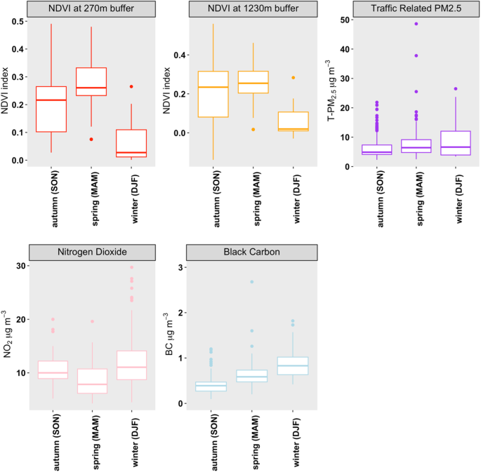
GPS data was also used to construct 48-hr activity spaces and calculate environmental exposures encountered within them [38]. Briefly, activity spaces are defined as the local areas that individuals interact with when they move around during their daily activities [45, 46]. We constructed activity spaces using Kernel Density Estimation (KDE) method for each individual and then calculated the following environmental exposures within them: walkability index score, Normalized Difference Vegetation Index (NDVI, greenness), parks and open spaces, traffic volume on primary roads, and road lengths (for primary and secondary roads combined and for minor streets). Data sources for these measures are listed in Table S3. Briefly, KDE integrates time and space to account for durations of time spent at certain locations and incorporates a distance decay kernel function to assign higher weight to environmental features closer to the locations where participants spent the most time in (compared to locations they passed through) using pre-defined bin (e.g., 25 m) and neighborhood sizes (e.g., 250 m) [45, 47]. Activity space calculations were conducted in ArcGIS Pro 2.5 (Esri, Redlands, CA).

Outdoor PM2.5 chemical speciation in study region

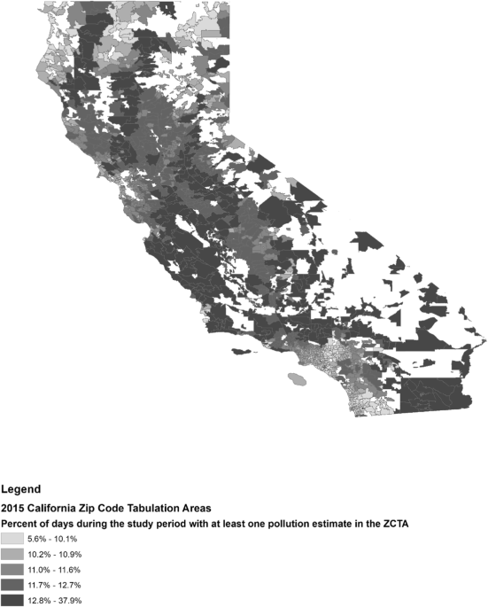
PM2.5 metals and carbonaceous components concentrations were available every third day from the Chemical Speciation Network (CSN) [48] at the Downtown Los Angeles monitoring station—the most proximal and central site in the study area—and were downloaded from the EPA Air Quality System. Then, the data was linked to personal monitoring 48- hr time periods based on the overlapping dates.

Data analysis

Descriptive statistics were first conducted to plot the distributions of all the variables (e.g., individual/residential environment data) for the participants. Then, using USEPA PMF5.0 model, source apportionment analysis was performed on personal PM2.5 measurements to identify main sources, along with their contributions to PM2.5 mass. Once sources were resolved, bivariate analysis was conducted between each PM2.5 source and several variables describing personal behaviors, indoor/outdoor sources, and time-activity patterns to confirm source identities and understand the personal drivers that affect PM2.5 exposures.

Descriptive analysis

Descriptive statistics were calculated in SAS 9.4 (SAS Institute Inc) to describe the distribution of personal PM2.5 mass concentration, elemental components and carbon fractions (used in final PMF analysis), questionnaire variables (home ventilation, time-activity patterns, indoor sources, etc.), and environmental exposures (residential or GPS-derived).

Source apportionment analysis

The USEPA PMF 5.0 model was used to resolve and identify major sources of PM2.5 and quantify their mass contributions using measured concentrations and sample-specific uncertainties as inputs. Briefly, the PMF model uses factor analysis to identify source contributions and profiles for a given number of sources through solving the following equation: [19, 20, 49]

$$_}=\mathop\limits_^_}_}+_}$$

(1)

where Xij represents the concentration of chemical component j in sample i, gik represents the mass contribution of factor k in sample i, fkj represents the loading of chemical component j on factor k, and eij is the residual error for sample i and species j.

The PMF model solves Eq. (1) by minimizing the sum of squares object function Q for a given number of factors k: [20, 49]

$$Q=\mathop\limits_^\mathop\limits_^\left[_}}_}}}\right]^$$

(2)

where uij is the uncertainty of species j in sample i. The model decomposes the concentrations matrix into a contributions g matrix and profiles f matrix and constrains results to be positive (or not significantly negative) [20, 50]. Each observation is individually weighted by its uncertainty in Eq. (2); therefore, samples with higher analytical uncertainties will have less influence on the solution.

Based on the PMF-calculated signal-to-noise ratio (S/N) indicating the degree of analytical noise relative to the concentration of each species [19], we categorized species as “Bad” (S/N ≤ 0.2, excluded from analysis), “Weak” (0.2 < S/N < 1, downweighted in the analysis), and “Strong” (S/N ≥ 1, retained). Although Pb and V had S/N < 0.2, they were included in the analysis as potentially important tracers of traffic and fuel oil, respectively, and set to “Weak.”

Of the 36 elemental and carbon species, the following 16 were finally included as “Strong” in the PMF analysis: BC, BrC, Ba, Ca, Cl, Cu, Fe, K, Mg, Mn, Na, Ni, S, Si, Ti, and Zn. We also included 9 “Weak” species as follows: Al, Br, Co, ETS, P, Pb, Se, Sr, and V. PM2.5 mass was designated as the total variable. An extra 10% modeling uncertainty was added to account for sampling or modeling errors not captured in the sample-specific analytical uncertainties [19]. Missing concentrations were replaced by species’ medians. One out of 213 (0.5%) samples were excluded as outliers based on multiple species’ concentrations.

Solutions with five to seven factors were scanned first to decide upon a reasonable factor number in a final model with 100 runs. Q values were checked for no undue influence from outliers and no local minimum solutions. Based on chemical loading profiles and prior knowledge, the optimal number of sources was selected which provided the most physically interpretable solution [50]. The convergent solution with the lowest Qrobust value (goodness-of-fit parameter excluding points with uncertainty-scaled residuals greater than 4) was selected [19]. Fpeak rotations, where positive F peak values sharpen the F matrix and negative values sharpen the G matrix were performed next to refine the solution. The optimal Fpeak value for solution rotation was chosen based on the smallest change in Q [19]. Residuals and R2’s for each species were checked for normality and model fit, respectively. Finally, diagnostics analysis of Displacement (DISP), Bootstrap (BS) (100 bootstraps, 0.6 minimum correlation), and Bootstrap-Displacement (BS-DISP) were performed to estimate the variability in the PMF solution under different scenarios. DISP focuses on effects of rotational ambiguity in the profiles or loadings; BS identifies whether there are a small set of observations that can disproportionately influence the solution; and BS-DISP includes effects of random errors and rotational ambiguity [19].

Bivariate confirmatory analysis of source identities and drivers

Bivariate analyses were conducted to further confirm source identities and examine trends in their mass contributions. Scatterplots, boxplots, and nonparametric statistics (Spearman correlations for continuous variables and Kruskal-Wallis test for categorical ones) were used to describe and test the relationships of select factors (selected from the literature and prior knowledge) with each source’s predicted mass contributions. These included demographics, time-activity patterns, home characteristics, indoor air pollution sources, and outdoor residential and activity space based environmental exposures as described earlier. Categorical variables with unbalanced values (≥85% of the records have one value) or with high missingness (≥80%) were dropped from further analysis.