1 Introduction

Recent advancements in artificial intelligence (AI) have opened up new opportunities for the fields of cognitive neuroscience and clinical brain health research. In this context, the EU Horizon 2020 funded project AI-Mind (www.ai-mind.eu) has been established, which aims at developing AI-based tools to estimate the risk of dementia for people affected by mild cognitive impairment. The project collects a comprehensive set of biomarkers, including blood samples, sociodemographic information, digital cognitive test scores, and electroencephalography (EEG) data. A combination of traditional machine learning (ML) and deep learning (DL)-based algorithms will be employed. While the former commonly provides improved transparency and integration of domain knowledge, the latter has the capacity to find patterns and extract features in complex and unstructured data beyond what can be obtained by hand-crafted features.

DL is a method in AI with potential to significantly transform healthcare services (Hinton, 2018). By processing data in multiple layers, DL learns representations with different levels of abstraction. Breakthroughs of DL include processing of images, video, speech, audio, and text (LeCun et al., 2015). Despite the progress in research and development, there are still significant gaps to be filled for deployment of AI in clinical practice, such as mitigating discriminatory bias and improving generalization to new populations (Kelly et al., 2019; Chen et al., 2023). In particular, AI systems trained on datasets with an underrepresentation of marginalized groups have an elevated risk of bias toward those groups (Rajpurkar et al., 2022). Furthermore, AI algorithms trained on data generated by a single system (e.g., when all imaging data are collected using the same camera with fixed settings) may exhibit single-source bias, resulting in a decrease in performance on inputs collected from other systems (Rajpurkar et al., 2022). For the AI-Mind project, such biases may pose challenges requiring particular considerations. While about two-thirds of dementia cases are in low-income and middle-income countries (LMICs), extrapolating predictive models developed in high-income countries to LMICs is not always feasible (Stephan et al., 2020). A technical prerequisite for extrapolating models to LMICs is the availability of hardware needed for data acquisition. As a neuroimaging modality, EEG is low-cost and mobile compared to magnetic resonance imaging and magnetoencephalography. Moreover, it does not require a dedicated isolated room. Extrapolation of EEG biomarkers to LMICs is thus not hindered by difficulties in installation of the acquisition hardware.

The recent progress of DL has significantly increased its relevance for EEG data analysis (Roy et al., 2019). Domains of application include emotion recognition (Houssein et al., 2022), driver drowsiness (Stancin et al., 2021; Mohammed et al., 2022), classification of alcoholic EEG (Farsi et al., 2021), epileptic seizure detection (Ahmad et al., 2022), mental disorders (de Bardeci et al., 2021), schizophrenia (Oh et al., 2019), major depressive disorder and bipolar disorder detection (Yasin et al., 2021), motor imagery and other brain computer interface (BCI)-related problems (Lotte et al., 2018; Abo Alzahab et al., 2021). Despite the attention of DL in EEG, little research has focused on issues relating to the cross-dataset setting and generalization (Wei et al., 2022). As AI-Mind will use EEG signals for its algorithm development, enabling our tools for deployment on multiple data acquisition systems and mitigating discriminatory bias, is a necessity.

However, a common limitation of many existing DL architectures occurring specifically to EEG is their inherent inability to handle a varied number of channels as input data (Wei et al., 2022). This lack of compatibility conflicts with the real-world high variety of EEG hardware and hinders training and deployment on heterogeneous datasets where both the number of electrodes and their positions on the scalp may vary. Hence, this challenge not only prevents integration of DL models into diverse EEG setups but also limits the inclusion of larger sample sizes as well as more heterogeneous and representative data. Moreover, evidence from clinical neurology research suggests that the number of channels used during EEG recording may have a significant impact on the data's ability to capture spatially limited phenomena (Hatlestad-Hall et al., 2023). The inability to handle this diversity originates from tensors such as matrices and vectors requiring fixed dimensions to be compatible from a linear algebraic perspective. To address this technical issue, this work aims at introducing a simple methodological framework which can be used in combination with current and future DL models to handle a varied number of electrodes. Here, two methods for scaling the data to fit into the DL model are used as baselines for comparison: (1) zero-filling missing channels and (2) applying spherical spline interpolation (Perrin et al., 1989).

There exist several techniques which may leverage external datasets to improve DL models, which we hypothesize will play a significant role in cross-dataset learning and generalization. Approaches such as unsupervised and self-supervised learning may be utilized even in the absence of the target of interest. Improvements may be in terms of, e.g., performance or generalization, and are considered to play an important role for data efficiency of DL (Hinton, 2018; Hendrycks et al., 2019; Banville et al., 2021). In the field of EEG research, Kostas et al. (2021) obtained improved results on multiple downstream datasets by using contrastive self-supervised learning on a large dataset for pre-training. Furthermore, Banville et al. (2021) successfully applied self-supervised learning to sleep staging and pathology detection. Another approach on heterogeneous EEG datasets is to use transfer learning, shown in the BEETL competition (Wei et al., 2022). Furthermore, a desired outcome of AI-Mind is to characterize brain networks from EEG data. While metrics from neuroscientific literature have known cognitive relevance (Stam et al., 2006), a DL methodology to obtain features of similar neurophysiological meaning seems non-trivial. This is due to features of DL being learned in a data-driven manner rather than human defined to capture the underlying neurophysiological phenomena. We hypothesize, however, that feature learning and pre-trained models may be viable alternatives.

The intended purposes for developing methods for handling a varied number of channels with possibly different positions on the scalp are (1) to enable the application of DL models on a range of existing and varied EEG systems. For clinical implementation, a highly desired property is to have a method which works on the EEG systems currently in use at different clinical centers around the world. The number of channels and channel locations are indeed varied, meaning that it is a necessity to handle this diversity, to maximize outreach and clinical usefulness; (2) to be able to pre-train or perform representation learning on heterogeneous and large amounts of data. There are many open-source datasets from a range of nationalities, pathologies, age groups, and cohorts. To generalize across such data, methods including pre-training and representation learning on multiple and heterogeneous datasets may be a step in the right direction, as it can lead to more robust and generalized features. Improving the robustness and generalization may in turn improve the fairness and equity of the developed AI models. This relevance extends to all medical use and integration of DL in EEG, including the generation of synthetic data (Goodfellow et al., 2014) and digital twins (Grieves and Vickers, 2017), and enabling of simulation techniques for improved clinical treatment selection. Indeed, developing methods to facilitate the evolution of such precision medicine approaches is essential. This study does not carry out such pre-training or representation learning but introduces a framework for enabling it to be performed in a larger scale, with a varied number of electrodes. Instead, this study conducts an initial evaluation to ascertain the efficacy or inadequacy of the framework.

Our framework is designed to be model agnostic, meaning that both current and future DL architectures can apply it with ease. The code is publicly available and may be used to develop customized implementations of the framework, or to combine it with other DL architectures. Furthermore, we aim to experimentally demonstrate that by applying our framework, the algorithm performance in itself remains the same.

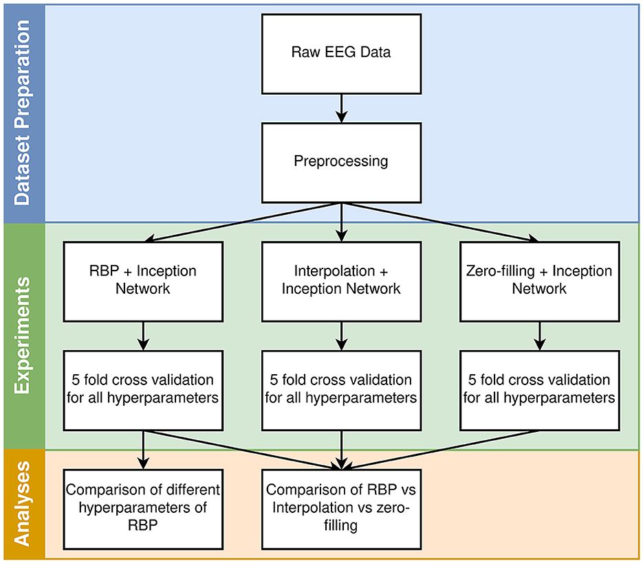
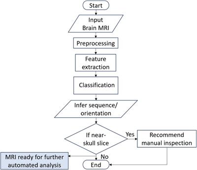
2 Materials and methods

In this section, the dataset, methods, models, and experiments are described. A high-level overview of the workflow is provided in Figure 1.

Figure 1. High-level overview of the workflow. The different hyperparameters for each model are described in Section 2.5.

2.1 Data

The data used for this study is an open-source dataset from Child Mind Institute (Alexander et al., 2017). It contains a large high-density EEG (129 electrodes) dataset from the age distribution 5–21 years, including male and female subjects, with varied brain pathologies. The objective of the DL models was to classify the sex of a subject, given the EEG data. After removing samples which did not fulfill the inclusion criteria for data quality (see Section 2.1.1), the dataset was balanced by down sampling the class in abundance, resulting in a final dataset with 1,788 subjects. Only the resting-state EEG data files were extracted. The first 30 s of the recordings were skipped as the first parts of the EEG are more likely to contain unwanted artifacts. The proceeding 10 s was used as input for the models. Only a single 10 s window was used per subject, and the splitting of data was thus made on subject level. The sampling frequency was kept at 500 Hz as in the original dataset.

2.1.1 Preprocessing

The raw data was preprocessed using an automated data cleaning pipeline developed in MATLAB, using functions from the EEGLAB toolbox (Delorme and Makeig, 2004). Channels with low-quality data were removed by iterative exclusion of signals with amplitude standard deviation SD>75μV or no amplitude variation at all. The EEG file was rejected if the number of excluded channels exceeded 39 (>30%). Line artifacts were removed with Zapline (de Cheveigné, 2020), and the signals were band-pass filtered between 1 and 45 Hz. Excluded channels were replaced with interpolated signals to ensure data dimension consistency. The channels were re-referenced to the average of all scalp channels. The pipeline is available at GitHub.

2.2 Inception network

The Inception network is a convolutional neural network (CNN) based architecture, which is the main building block of InceptionTime. Here, the Inception network is briefly described, and for further details on the architecture, the reader is referred to the original study (Ismail Fawaz et al., 2020).

An Inception network is composed of multiple Inception modules, with linear shortcut connections for every third Inception module. A key component of the Inception module is the bottleneck layer, which effectively computes linear combinations of the input time series. Furthermore, the Inception module applies filters of different lengths simultaneously on the same input time series, and resulting feature maps are aggregated by concatenation. After passing the data through all Inception modules, global average pooling is performed in the temporal dimension. Finally, while the original Inception network used a fully connected layer with softmax activation, this was changed to a single fully connected layer with sigmoid activation (Ismail Fawaz et al., 2020).

The hyperparameters of our Inception network was set as described in the original study. This includes a depth of six Inception modules, and 32 number of filters for all convolutional kernels in all Inception modules (Ismail Fawaz et al., 2020).

2.3 Methods for handling a varied number of channels

Three methods for handling a varied number of channels were tested on a binary classification problem, sex prediction. The three methods were (1) zero-filling, (2) spherical spline interpolation (Perrin et al., 1989), and our suggested new method (3) Region Based Pooling (RBP). Inception network (Ismail Fawaz et al., 2020) was the DL model used after zero-filling, interpolation, or applying RBP, with the exception that the final layer used scalar output and sigmoid as activation function for predictions.

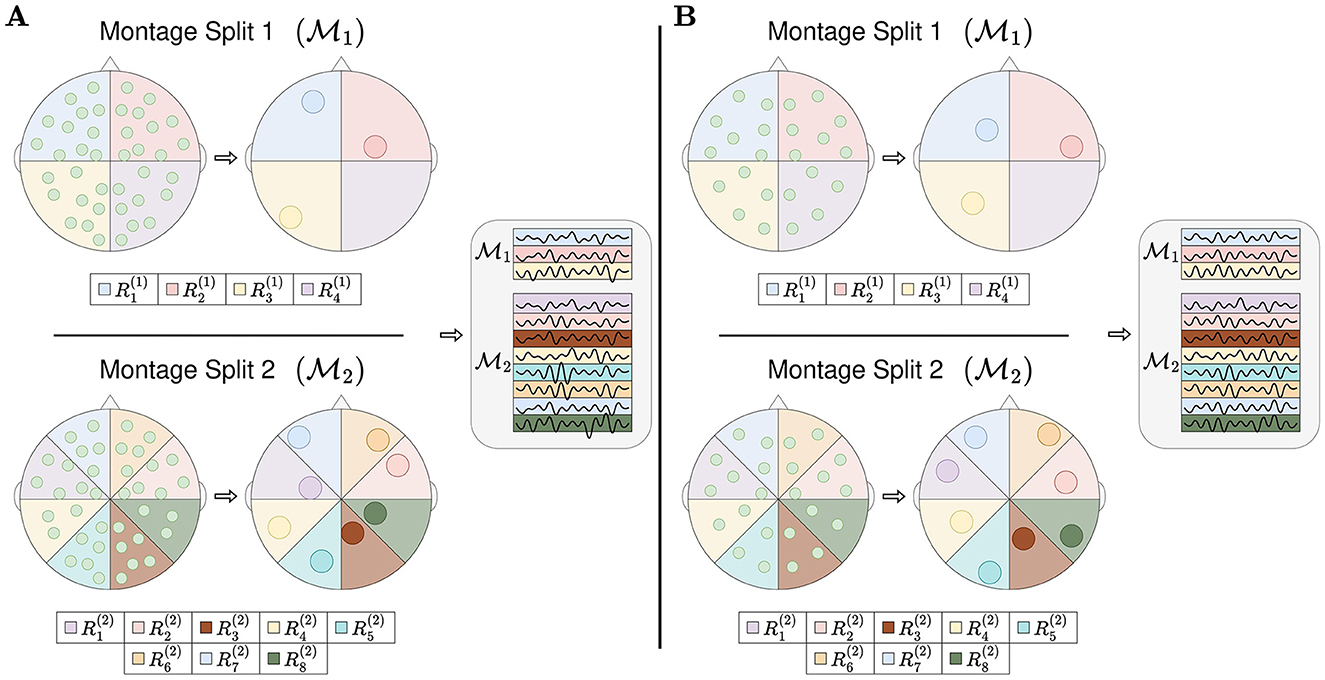
2.4 Region based pooling

RBP splits the topology of the EEG montage into regions, as illustrated in Figure 2. The channels within a single region are pooled into one or more region representations, and hence the name Region Based Pooling. To minimize the loss of information, multiple splits with different region formations are performed. RBP introduces three new optimization problems; (1) how to split the EEG montage into regions (both the number of montage splits and the algorithm separating the regions), (2) how to pool the channels within the same region, and (3) how to merge the outputs of the different montage splits. The proceeding two subsections intend to illustrate how the first two problems can be addressed and are meant as examples of implementation.

Figure 2. Region based pooling. The EEG montage is split into multiple regions. All channels in the same region are pooled into a region representation. Multiple montage splits may be performed, and the number of montage splits equals to two in this figure, M1 and M2. If there is at least one channel in all used regions, the mapping from channels into region representations can be made. This is illustrated as channel system A and channel system B have unequal numbers of channels with different channel locations, and they can both obtain region representations. After pooling channels into region representations, the region representations are stacked/row concatenated. The sequence of stacking represents an arbitrarily chosen design.

All RBP models in the experiments of this study merged the outputs of the montage splits by concatenation. Furthermore, all channels within the same region were merged to a single region representation. Finally, all region representations were normalized by subtracting the mean and dividing by the standard deviation in the temporal dimension.

2.4.1 Method for splitting into regions

A montage split is a region-based partitioning of the EEG montage. The set of all montage splits are denoted , where n is the number of montage splits. Each montage split contains multiple regions, Mi= ∀i∈, where the regions may or may not overlap. Furthermore, a montage split may or may not cover the entire EEG montage. Given a channel system C which is compatible with the partitioning, the j-th region of the i-th montage split Rj(i)∈Mi contains the channels Rj(i)⊃Rj(i)∩C, where Rj(i)∩C denotes the set of channels of channel system C, positioned within the boundaries of Rj(i).

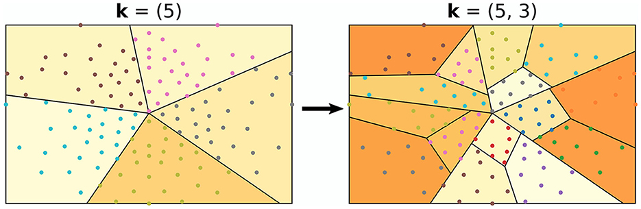
The algorithm used in all experiments for splitting the montage into regions is illustrated in Figure 3. It follows an iterative procedure and was designed to not have overlapping regions. Furthermore, all regions are used for all montage splits. The algorithm requires one to fix a split vector k=(k1,k2,...,kp)T∈ℕ2p, where the elements of k and p are design choices/hyperparameters. As a pre-step of the algorithm, all channel positions are mapped to 2D coordinates. Thereafter, the centroid of the channel positions is calculated, and a random angle is generated. With the centroid and the random angle as starting point and angle, k1−1 angles are computed such that the angles split the channels into k1 equally sized regions. Here, the size of a region refers to the number of channels within it. For all newly generated regions, the same procedure is repeated; (1) compute the centroid (2) generate a random angle, and (3) generate k2−1 angles such that k2 number of equally sized regions are formed. This iterative approach is executed either p times, or until the number of channels in the regions are too low, defined by a stopping criteria min_nodes.

Figure 3. Example of how the EEG montage may be split into regions. In this example, the split vector was set to k = (5, 3). This can be observed, as the montage was first split into five regions, followed by splitting those into three regions.

For the experiments, there were seven different split vectors, k = (3, 3, 3)T, k = (4, 2, 4)T, k = (2, 4, 2)T, k = (2, 2, 2, 2, 2)T, k = (3, 2, 3)T, k = (2, 3, 2)T, and k = (3, 4, 2)T. For each montage split, the selection of k was made by random sampling with equal probabilities. The stopping criteria was one of the hyperparameters for grid search and included min_nodes∈.

2.4.2 Pooling operations

To enable compatibility with a varied number of channels with possibly different channel positions, defining pooling mechanisms which can input and handle multivariate time series of different dimensions within the regions, is a prerequisite. That is, to apply mechanisms within the regions which can map a varied number of channels to a single region representation. Finding sophisticated mechanisms with this property may be crucial for RBP. This subsection presents several approaches for pooling mechanisms.

2.4.2.1 Average

The first pooling mechanism is to merge the channels within a region by computing its mean in channel dimension. This offers a simple and time-efficient method and aggregates the channels with equal contributions for computing region representations.

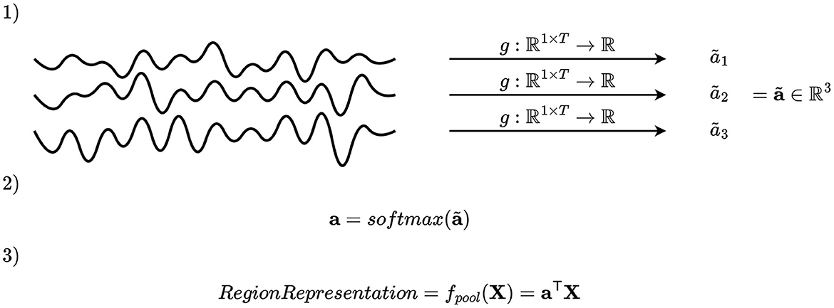
2.4.2.2 Channel attention

A second pooling mechanism is to select the key channels by first assigning an importance score, and secondly merge the channels by computing a weighted average based on the importance scores. Mathematically, this may be accomplished by defining a function g:ℝ1 × T → ℝ, where T denotes the number of time samples, applied on all time series within the region, and using the values obtained to compute coefficients of a linear combination, as illustrated in Figure 4. Applying g to each channel in a region gives an importance scalar for each channel, which is subsequently concatenated and passed to a softmax activation function, giving the channel attention vector of the i-th montage split and j-th region a(i,j)∈. The vectors a(i, j) have the properties that the entries are positive and sum to one due to the softmax activation function. After computing a(i, j), the channels of the i-th montage split and j-th region are pooled by weighted averaging fpool(i,j)(X,C)=a(i,j)TXRj(i)∩C, where XRj(i)∩C∈ℝ|Rj(i)∩C|×T are the EEG time series of all channels within the region.

Figure 4. Illustration of channel attention mechanism. An importance scalar is computed for each channel, and the attention vector is computed by applying softmax on a concatenation of these. The elements of the attention vector are used as coefficients to compute a linear combination of the channels.

ROCKET-based features: Random Convolutional Kernel Transform (ROCKET) (Dempster et al., 2020) is a highly efficient time series classifier, which obtained high performance in a short time frame in a multivariate time series classification bake off (Ruiz et al., 2021). For feature extraction, ROCKET applies a large number of diverse, random and non-trainable convolutional kernels, and computes the proportion of positive values and maximum value of the resulting feature maps. This was adopted as a pooling mechanism, where the proportion of positive values and max values of the feature maps were used for computing the importance score of a channel. From the num_kernels · 2 features, a trainable fully connected module with scalar output and specific to the i-th montage split and j-th region, FC(i, j):ℝnum_kernels·2 → ℝ, was applied. After computing the importance scores for all time series in the region, a softmax activation function was applied to obtain positive coefficients only, which sum to one. A desirable property of using non-trainable convolutional kernels is that the output feature maps (along with proportion of positive values and max values) are being computed only once per subject, prior to training. Therefore, the computational cost of a large number of convolutions may be justified by its property to be pre-computed.

The number of convolutional kernels was set to 1000, and the maximum receptive field in the temporal dimension to 250, which corresponds to half a second with the given sampling rate. This was based on computational feasibility, taking both time consumption and memory usage on limited hardware into account. Furthermore, no padding was used, in contrast to the original implementation. The ROCKET features were pre-computed prior to training, as the convolutional kernel weights were frozen, and the proportion of positive values and max values of the feature maps were thus constant per channel and subject during training. Furthermore, the ROCKET kernels were shared across all regions and montage splits to reduce runtime. The FC modules mapping the num_kernels·2 features to a single coefficient, used only a single fully connected layer with linear activation function. That is, for every subject, the importance score of the k-th channel in the j-th region of the i-th montage split prior to softmax normalization, was computed as g(i,j)(xk)=FC(i,j)(zk)=wi,jTzk, where wi,j∈ℝnum_kernels·2 is a trainable weight vector of the j-th region of the i-th montage split, xk∈ℝT is the time series of the k-th channel, and zk∈ℝnum_kernels·2 is the pre-computed ROCKET features of channel k.

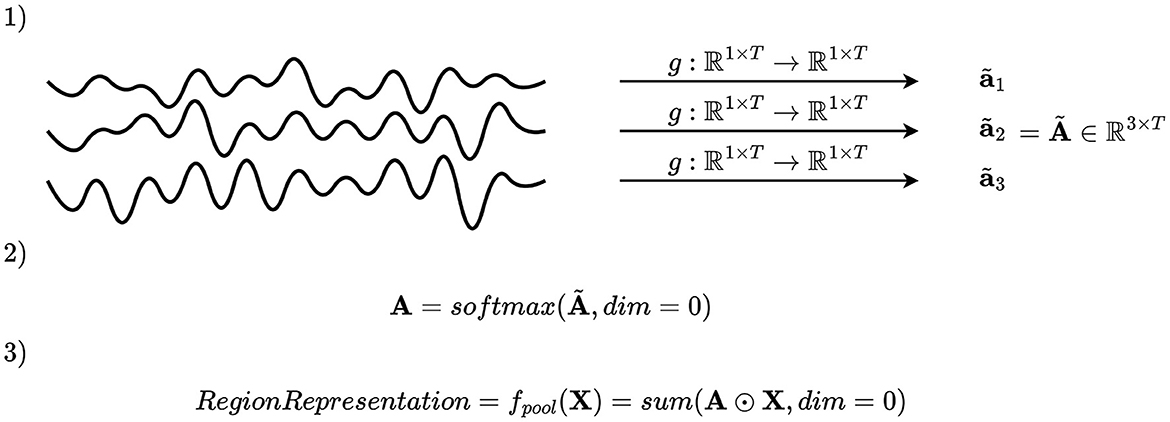
2.4.2.3 Continuous channel attention

Another possible pooling mechanism is to apply continuous channel attention, which is illustrated in Figure 5. In the channel attention mechanism explained in Section 2.4.2.2, it is impossible for the model to adapt its channel attention in time. Therefore, continuous channel attention is implemented by defining a function g:ℝ1 × T → ℝ1 × T, apply g to every channel, and apply softmax activation function in the channel dimension. That is, what was in Section 2.4.2.2 an attention vector of the j-th region in the i-th montage split a(i,j)∈ is replaced by an attention matrix A(i,j)∈}, where all elements are positive and each column sum to 1 due to the softmax activation function. The region representation of the j-th region in the i-th montage split is followingly computed as fpool(i,j)(X,C)=1T(A(i,j)⊙XRj(i)∩C), where 1 is a vector of ones, ⊙ is the Hadamard product (element-wise multiplication), and XRj(i)∩C∈ℝ|Rj(i)∩C|×T is the EEG data of the channels in Rj(i)∩C. This formulation is equivalent to applying a unique attention vector per time step.

Figure 5. Illustration of continuous channel attention. An importance scalar is computed for every channel and time step, and the attention matrix is computed by applying softmax on a concatenation of these in the channel dimension. The attention matrix is used to compute a linear combination of the channels per time step. That is, a new linear combination is computed for each time step, allowing the pooling mechanism to shift its attention through time.

In the experiments, an Inception network (Ismail Fawaz et al., 2020) was used as g. The depth of the architecture was set to two Inception modules, and the number of filters was set to two for all convolutional kernels and Inception modules. These hyperparameters were set smaller than in the original study due to high memory consumption.

2.4.2.4 Region based pooling with head region

With the pooling mechanisms described in Sections 2.4.2.1, 2.4.2.2 and 2.4.2.3, RBP is not able to tailor the region representations based on other regions. As this may be an important property to possess, RBP can be extended to Region Based Pooling with a Head Region, which is illustrated in Figure 6. A head-region is selected, which exhibits the property of being able to influence the aggregation of channels in non-head regions.

Figure 6. Region based pooling with a head region. The head region may influence how the channels in the non-head region should be aggregated. This is done by passing an embedding vector of the head region to the aggregation functions. By passing different embeddings to the different non-head regions, the head region is allowed to search for different features in the different spatial locations.

The region representation is computed as an aggregation of the channels, given a vector embedding of the head region. For every montage split Mi∈, a head region H(i)∈Mi is selected. The region representation of all non-head regions Rj(i)∈Mi\ is computed as

f(i,j)(X,C)=AGG(i,j)(XRj(i)∩C;si→Rj(i)) ∀j:Rj(i)∈Mi\,    (1) si→Rj(i)=fi→Rj(i)(XH(i)∩C),    (2)

where si→Rj(i) is the search vector embedding of the head region H(i) with relevance to region Rj(i)∈Mi\, fi→Rj(i) is the function mapping the channels of the head region to si→Rj(i), and AGG(i, j) is an aggregation function. The vector embedding of the head region may thus depend on the region to compute a region representation of. The motivation of this is that the head region systematically searches for certain characteristics in the other regions, and such characteristics may depend on the given regions.

The region representation of the head region was computed as in ROCKET channel attention, introduced in Section 2.4.2.2. The search embeddings si→Rj(i) were computed as

si→Rj(i)=[f1(i,j)(ZH(i)∩C)⊙σ(f2(i,j)(ZH(i)∩C))]1,    (3) f1(i,j)(ZH(i)∩C)=Wi,j(1)ZH(i)∩C,    (4) f2(i,j)(ZH(i)∩C)=Wi,j(2)ZH(i)∩C,    (5)

where σ is the softmax activation function computed in the channel dimension, ZH(i)∩C∈ℝnum_kernels·2×|H(i)∩C| is a concatenation of the ROCKET features, and Wi,j(1) and Wi,j(2) are trainable weight matrices of the search embedding function of region Rj(i). The use of softmax allows the search embedding to weight the different channels in the head region differently for each ROCKET feature. The region representation of region Rj(i)∈Mi\ are computed per subject as

AGG(i,j)(XRj(i)∩C;si→Rj(i))=a(i,j)TXRj(i)∩C,    (6) ak =exp{cos(f1(i,j)(zk),si→Rj(i))}∑c∈Rj(i)∩Cexp{cos(f1(i,j)(