TARVA is a pragmatic, prospective, multicentre, parallel-group, non-blinded RCT aiming to compare the clinical and cost effectiveness of TAR versus AF in patients with end-stage ankle osteoarthritis aged 50–85 years.

Participants were recruited in 17 UK hospitals, varying widely from district general hospitals to specialist orthopaedic hospitals. Participants were identified during routine clinic appointments or through screening of referral letters or clinic lists. Participants aged 50–85 years were recruited as this is the typical age range of patients with end-stage ankle OA eligible for surgical treatment. Eligibility criteria were patients with end-stage ankle osteoarthritis who the surgeon believes to be suitable for both TAR and AF (considering deformity, stability, bone quality, soft tissue envelope and neurovascular status), able to read and understand the Patient Information Sheet (PIS) and trial procedures, and willing and able to provide informed consent.

If eligible, the patient watched a bespoke trial video and read the PIS and a generic factsheet about ankle osteoarthritis and its treatment options. After receiving informed consent, magnetic resonance imaging (MRI) and preoperative assessment was conducted 14–30 days prior to surgery. MRI is performed as part of standard care and there were no other requirements for extra tests or hospital visits. Patients were then randomised to one of the surgical approaches. The randomisation process was performed using the Sealed Envelope™ randomisation service based on a minimisation algorithm. Three minimisation variables were used: surgeon, presence of osteoarthritis in the subtalar joint, and presence of osteoarthritis in the talonavicular joint (as determined by preoperative MRI). Patients were allocated 1:1 to the TAR and AF groups. Baseline measures were recorded at the preoperative assessment. All participating surgeons had performed at least 10 TARs and at least 10 AFs. In both TAR and AF, surgeons’ usual postoperative procedure was followed, including immobilisation type and weight-bearing status [21]. Follow-up visits were conducted at 12, 26 and 52 weeks. Further details on the trial are available in the trial protocol [21], statistical analysis plan [22] and results [20] papers.

Patients with osteoarthritis were involved in the design of the TARVA study and development of the participant information resources, and a patient representative attended Trial Steering Committee meetings. The public, patient organisations, and charities (Versus Arthritis) were actively involved throughout the trial via newsletters, annual meetings and their websites. Ethical approval was granted by the London Bloomsbury Research Ethics Committee (14/LO/0807), and clinical trial authorisation was given by the Medicines and Healthcare products Regulatory Agency. The trial sponsor was University College London, and the trial was registered with the Controlled Trials ISRCTN Registry (ISRCTN60672307).

A micro-costing approach, which is often used in surgical RCTs [23], was used to calculate the cost of surgery. Detailed information on surgery was collected in a purposely designed Case Report Form (CRF), including information on surgery duration, operating surgeon and his/her grade, type of devices, duration of hospital stays and duration of immobilisation. The average surgery duration in the TAR group was 121 min (range 60–244 min) versus 103 min (range 45–240 min) in the AF group. The average duration of hospital stay was 2.5 days (range 0–12) in the TAR group and 2.1 days (range 0–17) in the AF group. Immobilisation was prescribed by means of walking boot and/or plaster. Nineteen percent of patients in the TAR arm were allowed to weight bear within 2 weeks, compared with only 5% of patients in the AF arm. The use of a walking boot was assumed for the entire duration of immobilisation. Participants were wearing a boot for an average of 8.9 weeks (range 0–46) in the TAR group and an average of 13.8 weeks (range 0–52) in the AF group. The plaster was assumed to be changed every 6 weeks. Participants were wearing plaster for an average of 3 weeks (range 0–52) in the TAR group and an average of 4.6 weeks (range 0–26) in the AF arm. The cost of each component was calculated using the unit costs (Online Resource Table S1). Over 50% of all TAR implants used were fixed-bearing.

To collect data on healthcare resource use, we adapted a Client Service Receipt Inventory (CSRI) questionnaire, which participants completed at baseline and 12, 26 and 52 weeks post-operation. The questions related to the use of General Practice (GP) and community NHS services, inpatient stays, outpatient visits, accident and emergency (A&E) visits and social service use. The questionnaire was developed in collaboration with patient representatives. The unit costs were obtained from NHS Reference costs [24] and Unit Costs of Health and Social Care (see Online Resource Table S2) [25,26,27]. During the trial, a concomitant medications log was kept that recorded dosage, frequency and duration of each prescription. The medications were costed using the British National Formulary [28].

Participants also responded to the questions related to out-of-pocket payments, including transportation costs incurred in the receipt of care, equipment, mobility aids and home adaptations. We collected information on payments for parking, taxis, and bus and train journeys. For private car journeys, we collected information on the miles per journey and used fuel costs to obtain the cost of a journey. Equipment, mobility aids and home adaptations were paid for fully or partially by the PSS, or fully out-of-pocket.

Participants were also asked about their employment status, time they had to take off work due to problems with their ankle, and family and friends’ time off work or usual activities due to care. We used the human capital approach to estimate the cost of lost productivity in the TAR group versus the AF group. Unit costs were the average gross hourly earnings for men/women and full-time/part-time employees. To value family and friends’ time off work, we used the same approach; however, as no information on carers was collected, we were not able to distinguish by gender or employee status (full-time vs. part-time), and we therefore used gross average earnings of all employees in the UK. We included the cost of replacing an employee, but these results should be interpreted with caution as the cost comes from a private study and has not been confirmed by any peer-reviewed publications. All unit costs related to out-of-pocket payments and other wider costs are reported in Online Resource Table S3.

All costs are reported in 2018/2019 Great British Pounds (GBP), and, where needed, the costs were adjusted for inflation using the NHS cost inflation index (NHSCII) [27].

The outcome of the economic evaluation was quality-adjusted life-years (QALYs), which were calculated using the EQ-5D-5L index values. The EQ-5D-5L questionnaire was completed by patients at baseline and 12, 26 and 52 weeks post-operation. The EQ-5D-5L Crosswalk Index Value Calculator, which maps EQ-5D-5L to the EQ-5D-3L value set and is recommended by NICE [29], was used to estimate the index values. QALYs were calculated as the area under the curve using the standard methodology [30].

The protocol [21] specified secondary within-trial analysis taking the shape of cost-effectiveness analysis using a patient-reported outcome measure, the Manchester-Oxford Foot Questionnaire (MOXFQ) [31] walking/standing domain score at 52 weeks post-surgery. However, as the main results paper did not report statistically significant differences in MOXFQ walking/standing domain scores, we deviated from the protocol and did not conduct a cost-effectiveness analysis.

Statistical analysis was prespecified in a health economics analysis plan [32]. All analyses were based on ITT and corresponded to the analyses in the clinical-effectiveness paper [20]. We reported the mean cost and standard deviation (SD) of each component comprising the cost of surgery, and estimated the difference between the two groups using a linear regression model controlling for the presence of osteoarthritis in each of the two adjacent joints (subtalar and talonavicular) and adjusting for clustering at surgeon level. We then calculated the total cost of surgery and estimated the difference in total cost between the two groups using the same regression model as described above. We used bias-corrected bootstrapping (1000 iterations) to calculate 95% confidence intervals (CIs).

We report the mean and SD of the number of visits based on the type of healthcare resource use. We calculated the mean cost per patient for the TAR group versus the AF group by type of service at 12, 26 and 52 weeks post-operation. The difference in the number of visits and the difference in costs were estimated using the same regression model as described above for surgery cost components. One exception was the proportion of participants who reported inpatient admission, where we used a probit model.

We estimated mean index values at each time point for TAR versus AF, and the mean unadjusted QALYs from baseline to 52 weeks post-operation.

Total costs included costs of surgery, health care resource use, concomitant medications, and equipment, mobility aids and home adaptations paid for by the PSS. The difference in each cost component was analysed using a linear regression model controlling for the presence of osteoarthritis in each of the two adjacent joints and adjusting for clustering at the surgeon level. The difference in total costs was analysed using a similar model but, in addition, controlling for baseline healthcare resource use costs. We used bias-corrected bootstrapping (1000 iterations) to calculate 95% CIs.

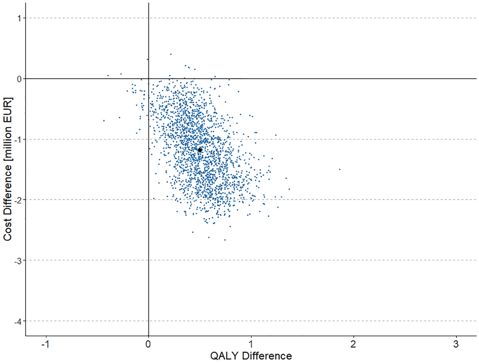
The mean per-participant differences in costs and QALYs were jointly estimated via bootstrapped seemingly unrelated regression with 1000 iterations to account for the correlation between costs and QALYs. We controlled for baseline healthcare resource use costs, baseline index values and minimisation variables, and adjusted for clustering at surgeon level. The incremental cost-effectiveness ratio (ICER) was calculated as the mean estimated difference in costs divided by the mean estimated difference in QALYs. We plotted the mean ICER and bootstrapping results on a cost-effectiveness plane (CEP). The bootstrapping results were used to calculate the cost-effectiveness acceptability curve (CEAC) [30], which shows the probability that TAR is cost effective compared with AF at 52 weeks for a range of cost-effectiveness thresholds for an additional QALY. As the time horizon was 52 weeks, costs and QALYs were not discounted. The analysis was complete case analysis, as <15% of participants were missing an ICER.

We conducted a post hoc subgroup analysis of total costs based on the type of TAR implant used: fixed-bearing versus mobile, as differences were noted in the clinical-effectiveness analysis [20]. Secondary within-trial analysis was conducted from the wider perspective, including out-of-pocket costs and the cost of productivity loss described in Sect. 2.2. Additional analysis also included the cost of replacing an employee, but as mentioned above, these results should be interpreted with caution. The wider perspective has not been applied in most studies that compared TAR and AF, but out-of-pocket costs are relevant to the condition and the intervention. As end-stage osteoarthritis can lead to disability, home adaptations and equipment are necessary for the patients and would lead to a reduction in working hours or retirement due to the condition.

Some patients received a different procedure from that for which they were randomised to. Therefore, we conducted a sensitivity analysis in the form of a per-protocol analysis, where we only included participants who received the surgery to which they were randomised.

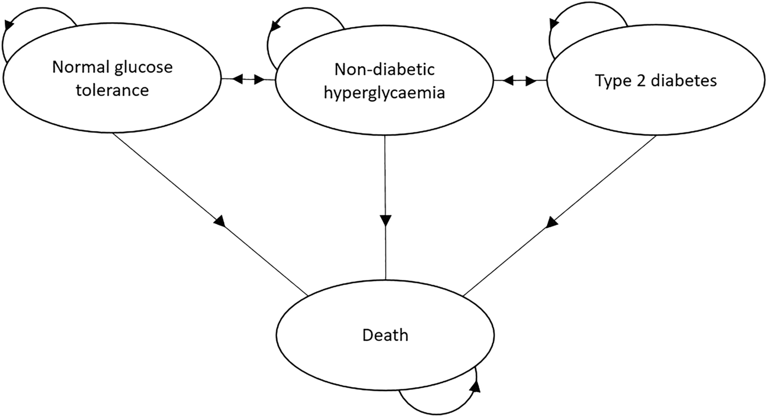
We built a decision model to extrapolate the trial results for the patients’ lifetime horizon, from the NHS and PSS perspective. We also constructed a simple Markov model using Microsoft Excel™ (Microsoft Corporation, Redmond, WA, USA), which simulates patients’ pathways after TAR or AF. The structure of the model is shown in Fig. 1.

The model was based on 1-year cycles, and there were 17 cycles in the model as the average life expectancy for a cohort aged 50–85 years was 17 years [33]. After surgery, patients can stay in good health, move to the revision state, or die. A patient can be in a revision state for 1 year only and then they move to ‘good health after revision’ or the death state. Transition probabilities are reported in Online Resource Tables S4 and S5.

Revision rates are based on the clinician’s opinion. The revision rate for TAR was assumed to be 1.2%, while the revision rate for AF was assumed to be 5% in the first 3 years (see Online Resource Table S5) and 0% thereafter. Revision is assumed to be AF in both the TAR and AF groups as this is more common in the UK. The death rate is based on the Public Health England Life Expectancy Calculator [34]. Each health state in the model was assigned a cost and a QALY outcome (as reported in Online Resource Table S6).

The costs assigned to the ‘good health’ and ‘good health after revision’ states are based on baseline resource use costs from the trial, whereas index values are based on the 52-week post-operation index values from the trial. We applied decrements to the index values due to revision based on the decrements reported by SooHoo and Kominski [17] as this was the only available source for these data. We assume that the revisions are successful and patients stay with the same quality of life for the remainder of their life. We discount costs and QALYs at the rate of 3.5%, as recommended by NICE [35].

We calculated an ICER at the lifetime horizon based on the model. Monte Carlo simulation was performed to address parameter uncertainty. We used gamma distribution for costs, beta distribution for index values, and Dirichlet distribution for transition probabilities. The distribution parameters are specified in Online Resource Table S7. Using the results from the simulation, we plotted the CEP and the CEAC.