Forty-seven CI users, between 20 and 79 years of age (mean = 60.9 years, SD = 12.1 years; median = 63.3 years; 46.8% female), were recruited from the University of Iowa Cochlear Implant Clinical Research Center. Demographic and audiological characteristics were obtained from clinical records. All the participants were neurologically normal. The average length of device use was 39.5 months (SD = 56.8 months). The average duration of deafness (i.e., patients’ experience of severe hearing loss) was 22.0 years (SD = 15.0 years). Five subjects were bilateral CI users. Among the remaining subjects, 66.1% had a CI in the right ear. Most of the current CI sample had some residual acoustic hearing usually in the low frequency ranges. A minority (23.7%) used bimodal configurations (electric stimulation in one ear and acoustic in the other) while the majority (76.3%) used a hybrid configuration (electric and acoustic stimulation within the same ear). Their hearing aids were in place during testing. The average threshold of low-frequency (i.e., 250 and 500 Hz) residual acoustic hearing in the better ear was 59.4 dB HL (SD = 20.5 dB HL). All CI users had post-lingual onset of deafness (i.e., onset of hearing loss later than 16 years old) and spoke American English as their primary language. See Supplementary Table 1 for the list of participants and their demographic information.

Most participants were tested during the same day as a clinical visit in which they received an annual audiological examination and device tuning. All participants were tested in the best-aided condition, which is the one they use most often in real life. All study procedures were reviewed and approved by the local Institutional Review Board. All the participants provided written informed consent.

All CI users performed the spectral ripple discrimination, temporal modulation detection, SFG, and speech in noise (AzBio) tasks. All tasks were performed in a double-walled sound booth using sound-field presentation from a single LOFT40, JBL speaker in the midline placed 1.5 m from the subject.

Performance on a sentence-in-noise task (AzBio: [40]) was used as a dependent variable in the later multiple linear regression analysis to predict CI individuals’ speech-in-noise ability. Our AzBio task was performed at +5 dB SNR at 70 dB SPL. Subjects heard a sentence and had to repeat it aloud. Outside of the sound booth, an audiologist counted the number of correctly repeated words. Performance was calculated as the ratio of correctly repeated words to the total number of words in all the twenty presented sentences.

Both the spectral ripple and temporal modulation tasks used an Updated Maximum-Likelihood (UML) adaptive procedure. On each trial, participants performed an oddball task in which they heard three sounds and indicated which differed from the other two in either spectral peak (i.e., the phase of spectral ripple) or modulation frequency (see below). Stimuli for both tasks were generated in MATLAB at the time of testing. The discrimination sequence used an Updated Maximum-Likelihood (UML) adaptive procedure [45]. UML is a Bayesian adaptive procedure which estimates a psychophysical function on each trial and uses the current estimate to identify the stimulus (e.g., the degree of ripple depth) that would be optimally informative to test on the next trial. This can lead to more robust estimates of performance with fewer trials than traditional staircase procedures.

Our implementation assumed a three-parameter logistic as the psychometric function with free parameters for threshold (which captures something akin to the just noticeable difference), slope (sensitivity), and guess rate. The crossover (expressed in terms of dB of depth) was used as our primary estimate of an individual’s perceptual fidelity on each dimension. That is, crossover indicates discrimination ability along spectral and temporal dimensions in each respective task.

Priors (mean and SD) of all three parameters were based on pilot data from 40 CI users. In the UML, the initial stimulus is governed by the priors, and after each response, the psychophysical function is refit. Subsequent trials are then adaptively generated based on the predictions of the UML procedure given the subject’s responses. Unlike traditional tasks, the UML procedure adaptively predicts what to test to best estimate an individual’s psychometric function.

For the spectral ripple task, the ripple stimulus was broadband noise that was sinusoidally modulated in log-frequency space. Ripple density was 1.25 ripples per octave—a low density meant to capture the kind of spectral shapes relevant to speech (e.g., the formants of a vowel) and avoid CI-related artifacts at high densities [43]. The amplitude depth of the ripples (in dB) was manipulated based on the UML predictions. On each trial, two standard sounds were created with a randomized starting location for the spectral peak, and the oddball was created with an inverted phase to be maximally distinct. Each trial’s standard and oddball intervals had the same ripple depth.

For the temporal modulation detection task, the stimulus was a five-component sound with frequencies at 1515, 2350, 3485, 5045, and 6990 Hz. The whole sound was sinusoidally amplitude modulated at a rate of 20 Hz, and the modulation depth was determined by UML prediction. Trials either had two modulated sounds, where the oddball was unmodulated, or two unmodulated sounds, where the oddball was modulated.

Stimuli for both tasks were 500 ms in duration and linearly ramped with a 50 ms rise/fall. To compensate for intensity differences in the modulated stimuli, root mean square values were equalized, and the presentation level was roved randomly across the three sounds by between −3 and +3 dB. This randomness should deter the use of loudness as a reliable cue.

The task was a 3-interval, 3-alternative forced-choice oddball detection paradigm. The task was implemented using Psychtoolbox 3 [46] in MATLAB (The Mathworks). On each trial, two standard stimuli and one oddball were played in random order with an ISI of 750 ms. A numbered box appeared on the computer screen as each stimulus played. Subjects were instructed to choose the token that differed from the other two. Responses could be made by numeric keypad or by mouse-click within the corresponding box on the screen. The UML approach allowed the tasks to be much shorter than traditional staircase measures; each task was 70 trials. Both tasks began with 4 practice trials to familiarize the subject with the procedure, and correct/incorrect feedback was given on every trial.

The SFG stimuli were generated as in [37]. Each time-segment contained a fixed number of components at random frequencies in log-frequency space. In trials containing a figure, a proportion of the components were constrained to remain the same over each time segment to create a figure with fixed frequency components that subjects were required to detect among a random background of frequency components. All the tone pips were constrained to be above 1 kHz so that even for subjects with residual low-frequency hearing, figure detection required only the electric range (and the acoustic hearing would most likely be unhelpful). The stimulus therefore assessed electrical grouping in all subjects, regardless of their hearing configuration. The spectral separation of elements was constrained to be at least a half octave to reduce the likelihood of frequency resolution abilities confounding the results. Figure 1A shows example spectrograms of ground-only and figure + ground stimuli. Figure 1B shows the electrodograms of example SFG stimuli, generated based on the 22-channel Cochlea device with the ACE sound coding strategy. Section 2.2 of Yang et al. [17] describes how the electrodograms are generated. Using the electrodograms, we compared integrated current levels between all the Ground-only and Figure+Ground stimuli in the 2–4 s period (where the emergence of a “figure” is expected). No significance difference was found between the current levels (Mann-Whitney Rank Sum test, p = 0.94), indicating that the overall current level difference could not be used to perform the task (Fig. 1C).

All stimuli were created using MATLAB software (The Mathworks) at a sampling rate of 44.1 kHz and 16-bit resolution. Extensive piloting with CI listeners was conducted to determine stimulus characteristics that were never associated with floor or ceiling effects. We used a stimulus that consisted of 50-ms segments, each containing eight frequency components. The whole stimulus was 4 s-long. For the first half (ground portion) of 40 segments, each segment was created from a selection of eight separate randomly selected frequencies drawn from a distribution of 145 components separated by 1/48th of an octave across 1–8 kHz. On a “ground” trial, the second half comprised 40 segments constructed in the same way as the first half. On a “figure” trial (see Fig. 1), the second half of 40 segments was constructed from components in which six of the eight stayed at the same frequency to create a “figure”. The other two components were selected at random frequencies.

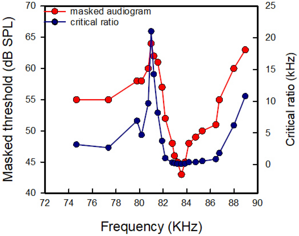
The SFG task was implemented in custom-written MATLAB scripts (The Mathworks) using Psychtoolbox 3 [46]. Instructions were presented via a computer monitor located 0.5 m in front of the subject at eye level. Sound levels were the same across subjects, presented at 70 dB SPL. At this presentation level, very few participants could use their residual acoustic hearing to hear the SFG stimuli; see the white areas in Fig. 2 that depicts the audibility zone of our SFG stimuli (i.e., above 70 dB SPL, above 1 kHz).

Residual acoustic hearing thresholds of all the participants represented in dB SPL as a function of stimulus frequency. The hearing thresholds were measured without a CI or hearing aids. The white areas depict the audibility zone of our SFG stimuli (i.e., above 70 dB SPL, above 1 kHz)

On each trial, participants saw the trial number displayed for 600 ms. This then cleared to display a fixation cross for 1 s before the start of the sound. After the sound and a 100 ms pause, a text prompt to respond was shown on the screen (‘Target? 1: Yes, 2: No’). Subjects then had up to 10 s to respond by a numeric keypad to indicate if a figure was detected. Once a response was recorded, the fixation cross was shown, and a delay of 600 ms occurred until the start of the next sound. One hundred and twenty trials were presented with a figure occurring in a random half; a break was given after 40 trials. One hundred and twenty unique different stimuli were pre-generated and presented in a random order. All the subjects were presented with the same set of 120 stimuli but in a different order.

Initial exploratory analyses related each predictor to each other and to AzBio performance using bivariate correlations. Our primary analysis related each predictor to speech perception performance on AzBio using multiple regression to assess the impact of SFG while controlling for the periphery. The final model is given in (1), in the syntax of the regression function in R (lm()).

$$Speech\; Perception \sim 1+SFG++TempMod$$

(1)

Here, Speech Perception is accuracy on the AzBio task, SFG is performance on the SFG task expressed in terms of d’. SpecRipple and TempMod refer to the crossover parameter of the psychophysical discrimination function expressed in dB of depth.