1. Introduction

Exoskeletons have enormous potential to enhance movement and to contribute to neuromuscular rehabilitation in persons with motor disorders such as stroke, cerebral palsy, and spinal cord injury (Sartori et al., 2016; Li et al., 2019, 2021; Liu et al., 2019; Zhang et al., 2019). Exoskeleton-assisted rehabilitation training involves the use of control algorithms aimed at improving muscle strength, neuroplasticity, and movement enhancement in users (Fujii et al., 2017). These control strategies can be classified into three types: passive control, triggered passive control, and assist-as-needed control (Marchal-Crespo and Reinkensmeyer, 2009; Meng et al., 2015; Proietti et al., 2016). Passive control refers to a technique in which the exoskeleton is in charge and guides the user to follow predefined trajectories or assistive forces/torques that have been extracted from healthy populations. The user is passive in the movement and does not actively control the exoskeleton. This type of control is often used in the initial stages of therapy to re-acquaint a limb to movement. Triggered passive control is a variant of passive control, where the user initiates the exoskeleton's assistance. Once activated, the user is again passive in the movement as the exoskeleton moves along pre-determined trajectories. This technique is often used to incorporate the brain-machine interface into the control process, providing assistance to individuals with irreversible impairments, such as tetraplegia (Proietti et al., 2016). Assist-as-needed control, also known as “user-in-charge” or “active control,” empowers the user to perform daily tasks with the aid of an exoskeleton. The exoskeleton provides assistance based on the user's ability and intention to generate torque, with the aim of promoting neuroplasticity and user autonomy. This active control technique is typically applied in persons with residual motor function (Chen et al., 2016; Durandau et al., 2017; Li et al., 2018; Yao et al., 2018). The primary focus of this paper is on active control techniques that seek to supplement the user's insufficient muscle contributions with assistance from an exoskeleton. Providing torque assistance based on the user's movement intention requires precise and robust decoding of motor function, which can be achieved through recording of underlying neuromuscular activities, such as brain and nerve signals and muscle electromyography (EMG) signals. EMG signals, which capture the electrical excitation of muscles, are a commonly used method for predicting joint torques, as they are easy to obtain and offer crucial insights into human motion (Sartori et al., 2018; Huang et al., 2019; Mounis et al., 2019).

Joint torque prediction is crucial in the control of exoskeleton-assisted rehabilitation and has frequently been achieved through two methods: physics-based neuromusculoskeletal (NMS) modeling and artificial neural networks (ANNs) (Pizzolato et al., 2015, 2019; Zhang et al., 2020, 2021). To improve prediction accuracy, ANNs have been integrated into NMS models in recent research. In our recent study (Zhang et al., 2022), an NMS solver-informed ANN model was developed to estimate ankle joint torque by combining features from an NMS model with a standard ANN, based on measured joint angles and muscle EMG signals during gait and isokinetic motions. This hybrid model was overall more accurate than the NMS or standard ANN models alone, but still showed poor prediction performance in one subject during gait, possibly due to incorporating less informative or misleading input features from the NMS model. This highlights the necessity of quantifying the uncertainty of joint torque predictions for safe and efficient human-exoskeleton interaction; accurate estimation of joint torque is crucial for determining the appropriate level of assistance from an exoskeleton.

A Bayesian Neural Network (BNN) is a well-established type of ANN for making predictions with uncertainties and has great potential in safe and efficient exoskeleton control (Cursi et al., 2021; Wei et al., 2021; Zhong et al., 2021). Unlike conventional ANNs (Cao et al., 2022b; Hu et al., 2022), BNNs incorporate probability distributions to represent prediction uncertainty and provide a probability distribution indicating the likelihood of different outcomes (Cursi et al., 2021). This characteristic makes BNNs useful for decision-making in various fields, including biomechanics, meteorology, and robotics. For instance, Zhong et al. (2021) developed a BNN-based framework for predicting the environmental context of lower limb prostheses. The quantified prediction uncertainty could lead to context recognition strategies that enhance reliable decision-making, efficient sensor fusion, and improved design of intelligent systems for various applications. Another popular technique for making predictions with uncertainties is the Gaussian Process (GP) (Chen et al., 2013; Yun et al., 2014; Maritz et al., 2018; Guo et al., 2019; Cao et al., 2022a). GP models the output as a Gaussian distribution with mean and covariance parameters, wherein the uncertainty is expressed by the covariance. Liang et al. (2021), for example, developed a GP model to estimate knee joint angles and uncertainties from EMG signals during walking and running movements. As both BNNs and GPs can estimate prediction uncertainty, it is of interest to compare the two methods in the context of safe and efficient human-exoskeleton interaction.

The objective of this study was thus to develop an NMS uncertainty-informed adaptive control framework for a knee exoskeleton. The framework aimed to provide accurate predictions of the user's knee flexion/extension (F/E) physiological torque, while also quantifying the level of estimation uncertainty. To achieve this, an NMS solver was employed to inform the machine learning models, which would subsequently adjust the assistance level based on the level of uncertainty. Another aim was to compare the predictions with uncertainties from the NMS solver-informed BNN (NMS-BNN) model with those from the NMS solver-informed GP (NMS-GP) model.

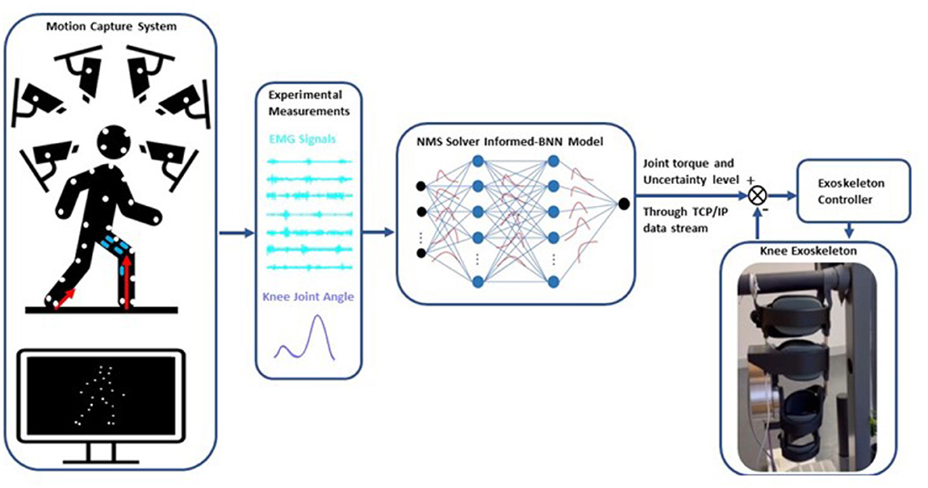
2. Methods

We developed an adaptive control framework for a knee exoskeleton based on an NMS-BNN model (Figure 1). The NMS-BNN takes two types of inputs: (1) experimental measurements—muscle signals and joint angles, and (2) informative physical features extracted from the underlying NMS solver, such as individual muscle force and joint torque. The NMS-BNN outputs knee joint torque with uncertainty quantification in the form of confidence bounds. The predicted torque with a specified confidence level is then used to control the assistive torque provided by the knee exoskeleton through a TCP/IP data stream. The study results consist of two key components: (1) an analysis of the NMS-BNN model's prediction accuracy and uncertainty, compared to the traditional NMS model and to the NMS-GP model; (2) an evaluation of the tracking performance of the assistive torque provided by the knee exoskeleton.

Figure 1. Schematic of the adaptive control framework for a knee exoskeleton based on an NMS solver-informed BNN (NMS-BNN) model. The inputs to the NMS-BNN include observed muscle signals and joint angles, as well as physical features derived from the NMS solver such as individual muscle force and joint torque. The NMS-BNN outputs knee joint torque with uncertainty quantification in the form of confidence bounds. The predicted torque with a specified confidence level is then used to control the assistive torque provided by the knee exoskeleton through a TCP/IP data stream.

2.1. Data collection and processing

Eight able-bodied subjects (sex: 4F/4M; height: 168.1 ± 9.4 cm; weight: 65.2 ± 17.8 kg; age: 29 ± 4 years) were recruited. The Swedish Ethical Review Authority (Dnr. 2020-02311) approved this study, and all subjects provided informed written consent documents. All participants were asked to do five movement types (Figure 2), specifically slow walking, normal walking, fast walking, sit-to-stand, and stand-to-sit. During the experiments, each movement was repeated at least ten times. The sequence of movements was randomized.

Figure 2. Experimental setup: subjects equipped with EMG sensors and markers, performed movements in an instrumented motion lab.

Surface EMG signals (aktos nano, myon, Schwarzenberg, Switzerland) from vastus medialis (VM), vastus lateralis (VL), rectus femoris (RF), semitendinosus (ST), biceps femoris (BF), gastrocnemius medialis (GM), and gastrocnemius lateralis (GL) of each participant's one randomly-selected leg were measured at 1,000 Hz. EMGs were post-processed by bandpass filtering (30–300 Hz), rectifying, low pass filtering (6 Hz), and normalizing to the maximum EMG value among all movement trials (Sartori et al., 2016; Pizzolato et al., 2017; Hoang et al., 2018).

Marker trajectories were recorded at 100 Hz using a 3D motion capture system (V16, Vicon, Oxford, UK), with marker placement based on the CGM2.3 model (Leboeuf et al., 2019). Ground reaction forces (GRFs) were measured at 100 Hz with three force plates (AMTI, MA, USA). Kinematics were calculated via inverse kinematics by solving a weighted least square optimization problem to minimize the discrepancy between virtual xi and measured xiexp marker trajectories (Lu and O'connor, 1999), Equation (1).

minq(∑iNθi||xiexp-xi||2),    (1)

where q represents the generalized coordinates of the model and θi is the weight of ith marker. Kinetics were computed via inverse dynamics by solving for joint torques in the dynamic equations of motion (Pandy, 2001) (Equation 2),

M(q)q¨+C(q,q˙)+G(q)+R(q)Fmt+Fe=0    (2)

where q,q˙,q¨ are the vector of generalized position, velocity and acceleration, respectively; M(q) is mass matrix and M(q)q¨ is a vector of inertial forces and torques; C(q,q˙) is the vector of centripetal and Coriolis forces and torques; G(q) is the vector of gravitational forces and torques; R(q) is the matrix of muscle moment arms; Fmt is a vector of musculotendon forces and R(q)Fmt is the vector of musculotendon torques; Fe is the vector of external force and torques (i.e., GRFs in this paper). A low-pass fourth-order zero-lag Butterworth filter (6 Hz) was used to filter joint kinematics and kinetics (Winter et al., 1974; Mantoan et al., 2015; Derrick et al., 2020).

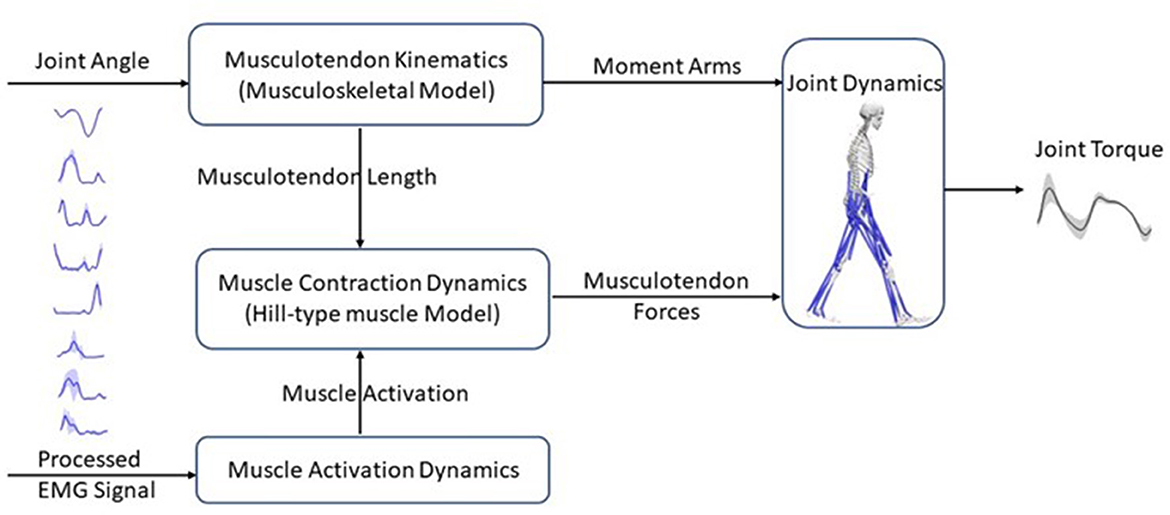
2.2. EMG-driven neuromusculoskeletal model

The EMG-driven NMS model used in this study was the open-source CEINMS model (Pizzolato et al., 2015) (Figure 3). This model includes four components: musculotendon kinematics, muscle activation dynamics, muscle contraction dynamics, and joint dynamics relationships (Sartori et al., 2011). The musculotendon kinematics component calculates moment arms and musculotendon lengths, while the muscle activation dynamics component computes muscle activation based on the available EMG information. The relationship between EMG excitation, e(t), and neural activation, u(t), is expressed in Equation (3) (Lloyd and Besier, 2003):

u(t)=α·e(t-τ)-β1·u(t-1)-β2·u(t-2)    (3)

where α is the muscle gain parameter, β1 and β2 are the recursive parameters [β1 = C1+C2, β2 = C1·C2, with |C1| < 1, |C2| < 1, and α − β1 − β2 = 1 for a stable solution (Lloyd and Besier, 2003; Buchanan et al., 2004; Pizzolato et al., 2015)], and τ is the electromechanical delay. Muscle activation, a(t), is described by Equation (4):

a(t)=eAu(t)-1eA-1    (4)

where A is the shape factor (Buchanan et al., 2004; Hoang et al., 2018).

Figure 3. Schematic structure of an EMG-driven neuromusculoskeletal model with four components: the musculotendon kinematics component calculates musculotendon lengths and moment arms; the muscle activation dynamics component uses the EMG information to compute muscle activation; the muscle contraction dynamics component, predicts musculotendon force using musculotendon length and muscle activation based on a Hill-type muscle model; and finally, the joint dynamics component computes joint torques with musculotendon forces and moment arms as inputs.

The muscle contraction dynamics component calculates the muscle force with a Hill-type muscle model, represented by Equation (5):

F=F0m[Fal(l)·Fv(v)·a+Fpl(l)+dp·v]cos(θ)    (5)

where F0m is the muscle's maximum isometric force, Fal(l) describes the relationship between active muscle force and fiber length l, Fpl(l) describes the relationship between passive muscle force and fiber length, Fv(v) describes the relationship between muscle force and fiber contraction velocity v, θ is the fiber pennation angle, and dp is the muscle damping parameter.

Finally, the joint dynamics component computes joint torque by multiplying muscle forces and moment arms.

The parameters were calibrated as outlined by Pizzolato et al. (2015), with optimal fiber length and tendon slack length adjusted within ±15% of initial values, coefficients C1 and C2 limited to values between −1 and 1, and parameter A bounded between (−3, 0). The maximum isometric force was determined using a strength coefficient with a range of 0.5 to 2.5. The optimization process focused on minimizing the error between predicted and actual joint torques (computed via inverse dynamics) during the calibration procedure. This optimization task was achieved by employing a simulated annealing algorithm, which iteratives to refine the parameter values. The algorithm was executed until the average change in the objective function's value reached a tolerance level of 10−5.

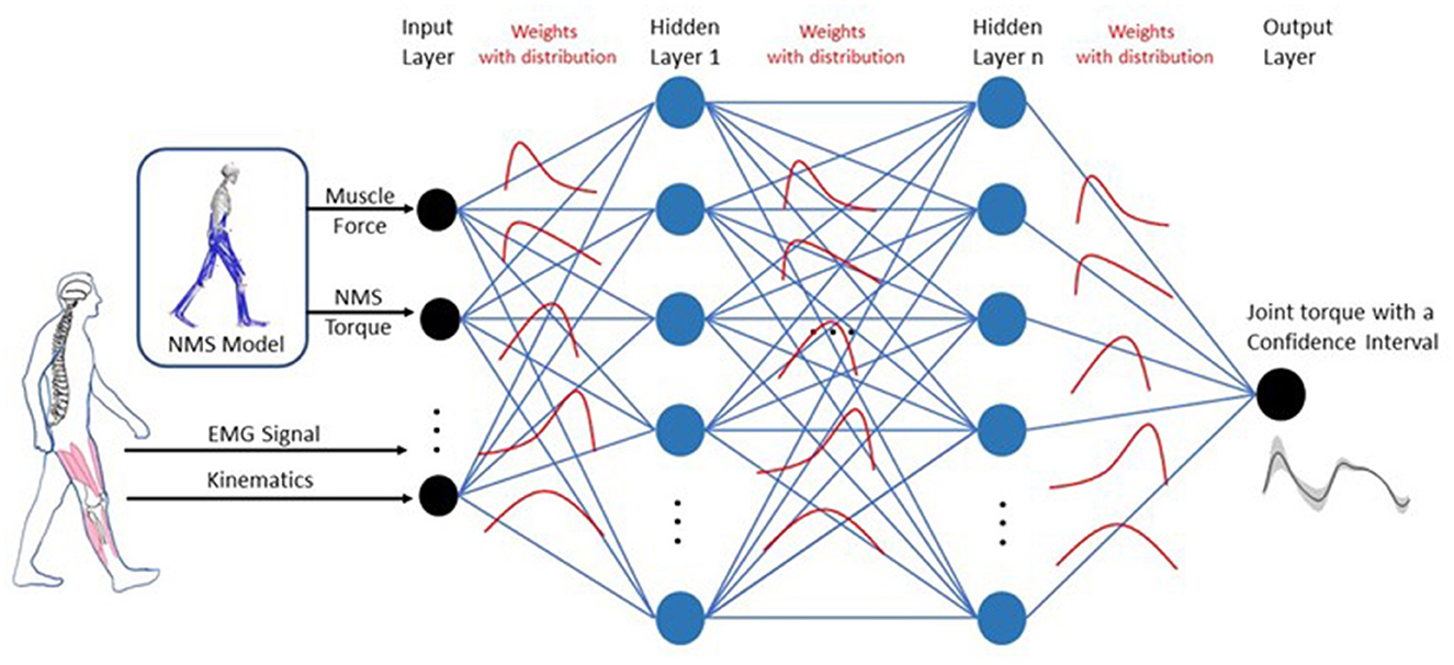
2.3. NMS-BNN model

The NMS-BNN models consist of an input neural layer, 3 hidden layers, and an output neural layer. The inputs, x=[x1,x2,…,xm]T where m = 21, were augmented with two types of features (Figure 4): (1) Muscle EMG signals and joint kinematics (knee F/E angle) from a 3D motion capture system, and (2) physical features such as muscle forces and NMS torque from an underlying NMS solver, to increase the model's accuracy by providing more information about the system being modeled. Each hidden layer has 40 neurons. The estimated knee torque with uncertainties bound was determined in the output layer.

Figure 4. Architecture for the NMS-BNN model. The NMS-BNN models consist of an input neural layer, 3 hidden layers, and an output neural layer. The inputs, x=[x1,x2,…,xm]T where m = 21, were augmented with two types of features: (1) Muscle EMG signals and joint kinematics from a 3D motion capture system, and (2) Physical features such as muscle forces and NMS torque from an underlying NMS solver, to increase the model's accuracy by providing more information about the system being modeled. Each hidden layer has 40 neurons. The estimated knee torque with uncertainties bound was determined in the output layer. Weights are treated as probability distributions rather than as single-point estimates as in standard neural networks. These distributions are used to reflect the uncertainty in weights and predictions.

In BNNs, weights are treated as probability distributions rather than as single point estimates, as in standard neural networks (Figure 4). These distributions are used to reflect the uncertainty in weights and predictions. The posterior probability of weights, P(W|X), is computed using Bayes theorem as follows (Equation 6):

P(W|X)=P(X|W)P(W)P(X)    (6)

where X is the data, P(X|W) represents the likelihood of the data given weights W, and P(W) is the prior probability of the weights. The denominator, P(X), represents the probability of the data, which is obtained by integrating the likelihood of the data given weights and the prior probability of weights over all possible values of weights, represented by Equation (7):

P(X)=∫P(X|W)P(W)dW    (7)

The BNN package TensorBNN, developed by Kronheim et al. (2022), was used in this study. The hyper-parameters of the BNN models were determined using a “coarse-to-fine” random search method (Bergstra and Bengio, 2012). During training, the mean square error was used as the loss function and a batch size of 32 was applied. Three hidden layers were included. Each hidden layer has 40 neurons with a tanh activation function. A Gaussian likelihood with a standard deviation of 0.1 was employed. Prior to sampling, the model was pre-trained using the AMSGrad optimizer with learning rates of 0.01, 0.001, and 0.0001, with a patience of 10. To obtain a point cloud of the posterior density of neural network parameters, Hamiltonian Monte Carlo (HMC) sampling was used to compute the likelihood function. HMC is a Markov chain Monte Carlo method that leverages a fictitious potential energy function derived from the posterior density of the neural network parameters. Numerical approximation was conducted using the leapfrog method, with the number of leapfrog steps and step size determining the distance traveled to the next proposed point. The number of steps for the HMC hyper-parameter sampler remained constant, while the step size was adapted using the Dual-Averaging algorithm based on the acceptance rate of the sample during 80% of the burn-in period. It is worth noting that selecting suitable values for the number of steps and step size can be challenging, and TensorBNN incorporates the parameter adapter algorithm to automatically optimize these parameters (Wang et al., 2013; Kronheim et al., 2022).

2.4. NMS-GP model

The NMS-GP model was developed using the same input data as the NMS-BNN model, which comprised experimentally obtained muscle signals and joint kinematics, as well as physical features such as muscle forces and NMS torque extracted from the underlying NMS solver. The NMS-GP model f(x) was specified by a mean function μ(x) and a covariance function k(x, x′), as expressed in equation (8) (Rasmussen, 2004).

f(x)~GP(μ(x),k(x,x ′))    (8)

where the mean function μ(x) provides an estimate of the expected value of the model at a given input, while the covariance function, also referred to as the kernel function, quantifies the similarity between two inputs. The Gaussian process model offers various kernel functions to capture the underlying structure of data. Among them, the radial basis function kernel (RBF) is widely used due to its smoothness and infinite differentiability, as shown in Equation (9),

k(x,x′)=exp(-|x-x′|22l2)    (9)

where l controls the length-scale of the kernel, and |x − x′| is the Euclidean distance between inputs x and x′.

Another popular kernel function is the Matern kernel, which is a generalization of the RBF kernel and is defined as Equation (10),

k(x,x′)=21-νΓ(ν)(2νl|x-x′|)νKν(2νl|x-x′|)    (10)

where ν determines the smoothness of the kernel, Kν is the modified Bessel function, Γ(ν) is the Gamma function, and l controls the scale of the kernel.

For modeling noise in data, the White Noise Kernel, as shown in Equation (11), is commonly used,

k(x,x′)=σ2δ(x-x′)    (11)

where σ2 is the noise variance parameter that determines the amplitude of the noise, and δ(x − x′) is the Dirac delta function. This function equals one when x = x′ and zero otherwise, ensuring that the kernel function is non-zero only at the diagonal of the input space.

The Linear kernel is another widely used kernel that models a linear relationship between the input and output variables. Specifically, it can be formulated as depicted in Equation (12):

k(x,x′)=σ2xTx′    (12)

where σ2 represents the variance parameter.

In Gaussian process modeling, the combination of different kernel functions can improve the performance of the model. In this regard, we selected a combination of Matern, White Noise, and Linear kernels after conducting extensive testing to obtain the most accurate predictions. The Matern kernel was used to capture non-linear patterns, while the White Noise kernel accounted for measurement errors and uncertainty, and the Linear kernel modeled linear relationships between the input and output variables. Hyperparameters such as length scale, signal variance, noise variance, and others were optimized during the training process to enhance the model's performance. In the Matern kernel, we set ν to 3/2, and the length scale was bounded between the range of (0.01, 200), with variance confined within the range of (10−3, 105). Similarly, the White Noise kernel had a noise variance bounded between (0.03, 100), while the Linear kernel had a variance range of (10−3, 105).

2.5. Knee exoskeleton

The knee exoskeleton hardware consists of a drive unit (Gen.1, Maxon, Switzerland), a 3D-printed thigh-shank frame, and thigh and shank straps (Orliman 94260, Spain). The drive unit features a brushless DC motor (EC90 flat), a MILE encoder with 4,096 counts per turn, a three-stage planetary gearbox with an 18-bit SSI absolute encoder, and an EPOS4 position controller. The drive unit is capable of providing a continuous torque of 54 Nm and a maximum torque of 120 Nm on a 20% duty cycle. The system can operate on a DC power supply ranging from 10 to 50vV and its actuation speed can reach up to 22 rpm.

2.6. Evaluation protocol 2.6.1. Joint torque prediction

The prediction accuracy of the knee joint torque for NMS, NMS-GP, and NMS-BNN models was investigated. The uncertainty of the predicted torque by NMS-GP and NMS-BNN models was also analyzed. The prediction accuracy and uncertainty quantification was compared in five cases: Gaitslow, Gaitself, Gaitfast, SitToStand, and StandToSit, which were trained using data from each movement separately. NMS-GP and NMS-BNN models were trained using 80% of the data and evaluated on the remaining data, while NMS models were calibrated using three trials of each movement and tested on the same data as NMS-GP and NMS-BNN models. The input data from each trial consisted of approximately 100 time-series data points and 21 dimensions.

Two prediction error metrics were evaluated: the Normalized Root Mean Square Error (NRMSE, ENRMS) and the Root Mean Square Error (RMSE, ERMS). A low prediction error indicated a high prediction accuracy. NRMSE was calculated by dividing the RMSE (between the predicted and actual torque) by the range of joint torque observed during the corresponding motion:

ERMS=1N∑n=1N(yp,n-yn)2    (13) ENRMS=ERMS(ymax-ymin)×100%    (14)

where yn and yp,n are the measured/actual and predicted torque respectively; and ymin and ymax are the minimum and maximum measured torque in corresponding movements. The RMSE and NRMSE were calculated for each subject and the average was obtained across eight subjects. The results section presents the average values of RMSE and NRMSE.

The normality of the data distribution was evaluated using Shapiro-Wilk tests (p < 0.05 significance level). To determine the differences among the NRMSEs and RMSEs estimated by the three approaches, pairwise comparisons were performed using either paired t-tests for normally distributed data or Wilcoxon signed-rank tests for non-normally distributed data, both with Bonferroni correction applied and significance level of p < 0.05.

The uncertainty of the predicted torque by NMS-GP and NMS-BNN models was quantified by using a 95% confidence level (CL), which means that there is a 95% probability that the true value of the function being modeled falls within the predicted interval. A high uncertainty value indicates low confidence in the predicted value.

2.6.2. Exoskeleton assistive torque tracking performance

We also evaluate the tracking performance of the knee exoskeleton's assistive torque provided by the adaptive control framework during five daily activities by using the two metrics: NRMSE and RMSE (between desired and actual torque provided by the knee exoskeleton). The assistance level AL of the knee torque provided by the adaptive control framework is adapted/determined by the uncertainties U quantified by the NMS-BNN model, as described by the following equation:

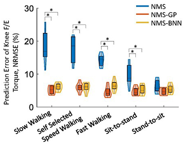
AL={0.8if U<0.050.6if 0.05≤U<0.10.4if 0.1≤U<0.150.3if 0.15≤U<0.20.1if U≥0.2    (15) 3. Results 3.1. Joint torque prediction

Overall, both NMS-BNN and NMS-GP models accurately predicted knee joint torque with relatively low error (RMSE: NMS-GP ≤ 0.05 Nm/kg, NMS-BNN ≤ 0.07 Nm/kg; NRMSE: NMS-GP ≤ 5.9%, NMS-BNN ≤ 6.8%). The errors were considerably lower than those of NMS models (RMSE: ≤ 0.14 Nm/kg, NRMSE: ≤ 18.3%, Figures 5, 6).

Figure 5. The distributions of NRMSE between estimated and measured/actual knee joint torques across subjects in NMS, NMS-GP, and NMS-BNN models during five daily activities. The violin plots depict the probability distributions of NRMSE using kernel density plots, and the box plots represent the minimum, lower quartile, median, upper quartile, and maximum values of NRMSE. A significant difference between any two models is indicated by an asterisk (*), based on paired t-test (for normally distributed data) or Wilcoxon signed-rank test (for non-normally distributed data) with Bonferroni correction.

Figure 6. The distributions of RMSE between estimated and measured/actual knee joint torques across subjects in NMS, NMS-GP, and NMS-BNN models during five daily activities. The violin plots depict the probability distributions of NRMSE using kernel density plots, and the box plots represent the minimum, lower quartile, median, upper quartile, and maximum values of NRMSE. A significant difference between any two models is indicated by an asterisk (*), based on paired t-test (for normally distributed data) or Wilcoxon signed-rank test (for non-normally distributed data) with Bonferroni correction.

The NRMSE prediction error for the NMS-GP and NMS-BNN models was significantly lower than that of the NMS models in all cases, except the StandToSit case (Gaitslow: p < 0.01 and p < 0.01; Gaitself: p < 0.01 and p < 0.01; Gaitfast: p < 0.01 and p < 0.01, SitToStand: p < 0.01 and p < 0.01, StandToSit: p = 0.08 and p = 1.45; Figure 5). Similar findings were also observed in the RMSE.

Among the NRMSE predicted by NMS models in five cases, the NRMSE in the StandToSit case was the lowest (≤ 7.2%). No significant differences were observed in the StandToSit case among NMS, NMS-GP, and NMS-BNN models (NMS: ≤ 7.2%, NMS-GP: ≤ 5.5%; NMS-BNN: ≤ 6.8%).

Both the NMS-GP and NMS-BNN models had relatively high uncertainties in the predicted knee torque at the beginning of each movement, particularly in the Gaitself case (Figure 7A). In the NMS-GP model, high uncertainties were observed during terminal stance and terminal swing in the Gaitself case. On the other hand, the NMS-BNN model had high uncertaint