Based on medical theory, the upper limb rehabilitation robot drives the affected limb to carry out scientific and effective training (Xu et al., 2011), so that the patient's motor function can be recovered better (Lin et al., 2003). According to the process of patient rehabilitation, the rehabilitation training stage of upper limb rehabilitation robot includes passive training (Lizheng et al., 2015), robot-assisted training (Chang and Kim, 2013) and resistance training (Song et al., 2014). During passive rehabilitation training, the joints of rehabilitation robot are required to have high stiffness to ensure the stability and high bandwidth of closed-loop position control, so as to drive the limbs of patients to reach the specified position accurately (Gopura et al., 2016). In the stage of assisted and resistance training, the rehabilitation robot must have good flexibility and exert different forces on the patient's limbs to ensure the safety and comfort of the rehabilitation process (Marchal-Crespo and Reinkensmeyer, 2009). It can be seen that at different stages of rehabilitation training, the driving joints of the rehabilitation robot need to have different stiffness (Ma et al., 2016). The traditional robot usually collects a large number of position, torque, speed and other data by increasing the type and number of sensors on the basis of rigid driving joints (Palazzolo et al., 2019), and then designs a controller that can process these data effectively, so as to achieve the effect of controlling the impedance of the rehabilitation robot (Yuan et al., 2013). This requires that the sensors, driving and control circuits of the rehabilitation robot run fast enough, and the system needs to establish an accurate dynamic model (Cestari et al., 2014). For example, the biped robot designed by Hubicki et al. (2018) uses inertial measurement units, encoders and other sensors to collect large amounts of data, and then processes these data through algorithms to achieve stable control effects. The driving joint of the traditional rehabilitation robot is not inherently compliant and cannot store energy, which leads to its inability to absorb the energy of the instantaneous impact (Caldwell et al., 2015). In recent years, some scholars have developed a variety of rehabilitation robots with variable stiffness joints instead of rigid joints. Vanderborgh et al. summarized the variable impedance actuators, and classified it into active impedance by control, inherent compliance and damping actuators, inertial actuators, etc. based on the principle of variable stiffness and impedance (Vanderborght et al., 2013). Yi et al. designed a variable stiffness joint of exoskeleton (Yi et al., 2018). Yang et al. used a variable stiffness rehabilitation robot to perform elbow rehabilitation training for stroke patients (Yang et al., 2021). Baser and Kizilhan designed a wearable ankle exoskeleton with variable stiffness (Baser and Kizilhan, 2018).

According to the working principle, the working principle of variable stiffness actuator (VSA) can be divided into variable lever arm, special curved surface, changing the number of elastic elements and so on. The way of changing lever arm is to change the transmission ratio between load and spring according to the proportion of lever arm. It is mainly composed of load point, pivot and spring contact point. Changing any position can adjust the stiffness of the mechanism. For example, Chaichaowarat designed a variable stiffness spring mechanism, which is composed of a slider, a roller and an adjustable unsupported length leaf spring. The adjustment of the slider position changes the spring contact point, thus obtaining the variable stiffness characteristics (Chaichaowarat et al., 2021). Similar variable stiffness actuators include AWAS-I (Jafari et al., 2010), AWAS-II (Jafari et al., 2014), COMPACT-VSA (Tsagarakis et al., 2011), etc. In the variable stiffness principle of special curved surface, the variable stiffness mechanism is connected in series between the reducer and the output shaft of the joint. The stiffness control motor changes the relative position of the cam disc to control the pretension force of the spring to adjust the stiffness of the joint. For example, the FSJ joint developed by Wolf, when the joint is subjected to passive torque load or the spring preload is changed, the cam disc rotates relatively, the spring is compressed, and the stiffness of the joint changes (Wolf et al., 2016). Similar special surface variable stiffness actuators include MESTRAN (Hung Vu et al., 2011), VSM (Sun et al., 2018) and SJM-II (Park and Song, 2010). Some variable stiffness joints adjust their stiffness by changing the number of elastic elements. In the discrete variable stiffness actuator designed by Hussain, the spring set is connected in series between the drive motor and the load end. The springs are controlled by the clutch, respectively. The on-off of the clutch can be realized by changing the number of spring connections (Hussain et al., 2021). In addition, there are other methods. For example, Garabini et al. designed a soft robots that mimic the neuromusculoskeletal system, which reproduces many of the characteristics of an agonistic-antagonistic muscular pair acting on a joint (Garabini et al., 2017). For the variable lever arm type variable stiffness joint, the torque curve depends on the length of the lever. If the length of the lever is increased, the volume of the mechanism will increase accordingly. For the variable number of elastic elements type, the volume of the mechanism will also increase due to the number of elastic elements. The ideal asymptote torque curve can be obtained only by changing the contour of the special surface, which is easier to achieve miniaturization in terms of volume and weight. Therefore, the principle of variable stiffness of the special curved surface will be used in this paper.

In terms of control, variable stiffness joints operate in a large stiffness range. In the case of low stiffness, vibration is often accompanied, and its torque response performance is also affected (Albu-Schaffer et al., 2010), which reduces the safety of human-machine interaction in rehabilitation training. To solve such problems, Liu investigated a closed-loop torque controlled variable stiffness actuator (VSA) combined with a disturbance observer, and a better dynamic response with high and low stiffness was achieved (Liu et al., 2021). Albu-Schaffer proposed a general variable stiffness joint model for nonlinear control design, and then designed a simple gain scheduling state feedback controller for active vibration reduction of weak damping joints (Albu-Schaffer et al., 2010). Misgeld designed a gain scheduling torque controller to improve the human-machine interaction characteristics of the joint. The eigenvalue of the gain scheduling is determined by the zeros and poles of the multi-channel H∞-control strategy, which can perform gain-scheduled control on multiple stiffness values of the joint in discrete time (Misgeld et al., 2017). In the interactive control of the manipulator, the gradient of the gain scheduled variable hyperplane is adjusted according to the real-time identified environmental stiffness to achieve stable position and torque control in different environments (Iwasaki et al., 2002). Mengacci et al. designed an iterative learning control scheme based on torque by decoupling the motion/stiffness of the articulated soft robot and learning the expected action of the robot, and accurately controlled the position trajectory of the articulated soft robot without changing the flexibility of the articulated soft robot. In this paper, the PID control scheme based on BP neural network is adopted to improve the torque response speed of variable stiffness actuator under different stiffness conditions (Mengacci et al., 2020).

In this paper, based on the existing research, a variable stiffness joint used in upper limb rehabilitation training is designed to improve the safety and comfort of the rehabilitation process. Compared with the previous work, the contributions of this paper can be summarized as follows.

(1) From the mechanical design point of view, the joint adopts the variable stiffness principle based special curved surface. The trapezoidal lead screw in the variable stiffness module has a self-locking function, and the stiffness can be maintained without the continuous output torque of the motor.

(2) From the control algorithm point of view, the PID control based on BP neural network is adopted to improve the torque control response performance of the elbow joint rehabilitation robot driven by variable stiffness joints under low stiffness by adjusting the gain parameters under different stiffness.

(3) Based on the principle of variable stiffness, this paper designs a variable stiffness joint for the elbow joint, and combines the PID control method based on BP neural network to build the experimental platform of the variable stiffness elbow joint rehabilitation robot, and the isotonic centripetal resistance training experiment of elbow joint is carried out to verify the effect of BP neural network PID torque control.

The rest of this paper is organized as follows: the second section introduces the mechanical design of the variable stiffness joint based on principle of special curved surface. The third section establishes the dynamic model of the joint, studies the PID control method based on BP neural network, and conducts simulation verification. The fourth section builds an experimental platform for a variable stiffness elbow joint rehabilitation robot, and takes the elbow joint isotonic centripetal resistance training as an example to verify the effect of BP neural network PID torque control. The fifth section is conclusions and discussions.

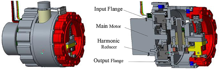
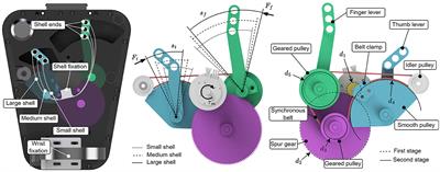
As shown in Figure 1, the overall size of the variable stiffness joint designed in this paper is 500*110*137.5mm, and the total mass is 1.5 kg. According to the structure and function, the mechanism can be divided into main drive module and variable stiffness module. The main drive module provides the output torque, and the variable stiffness module adjusts the joint output stiffness.

Figure 1. Variable stiffness joint model.

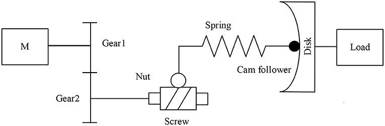
The main drive module includes a main motor and a harmonic reducer. The main motor is a brushless DC motor with a rated torque of 269 mNm, and the reduction ratio of the harmonic reducer is 100:1. Figure 2 is the schematic diagram of the variable stiffness module mechanism. The stiffness adjustment motor drives a pair of gears to rotate, the gears drive the trapezoidal lead screw to rotate, the lead screw nut moves forward, the spring is compressed, and then the cam rotates to adjust the joint stiffness.

Figure 2. Schematic diagram of variable stiffness module mechanism.

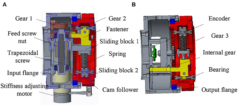
The specific variable stiffness module is shown in Figure 3A. The left is the input flange connecting the main drive module, and the right is the output flange connecting the load. The input flange and output flange are supported by cross roller bearings. The driving source of the variable stiffness module is a brushless DC motor with a rated torque of 10.8 mNm. The output of the motor is connected with a planetary reducer. The stiffness adjustment motor is installed on the input flange. The output of the reducer drives the gear 1 to rotate, and one end of the gear 2 is meshed with the gear 1, the other end of the gear 2 is connected with the trapezoidal lead screw. The trapezoidal screw rotates to push the screw nut forward. Due to the introduction of trapezoidal lead screw, the variable stiffness module has self-locking function. So, the stiffness adjustment motor does not need to output torque while maintaining the compression of spring to reduce energy consumption. The slide block 1 installed on the right side of the lead screw nut moves forward and compresses the upper end of the spring. The lower end of the spring is connected with the sliding block 2, and a cam follower is installed on the sliding block 2. The cam follower is tangent to the cam contour in the output flange and transmits the spring force to the output flange.

Figure 3. Three-dimensional model of variable stiffness joint (A) Sectional view 1 of variable stiffness module (B) Sectional view 2 of variable stiffness module.

In addition, as shown in Figure 3B, a rotary encoder is installed on the input flange, and the magnetic steel of the encoder is installed in the gear 3. An internal gear groove is designed in the output flange to mesh with gear 3. 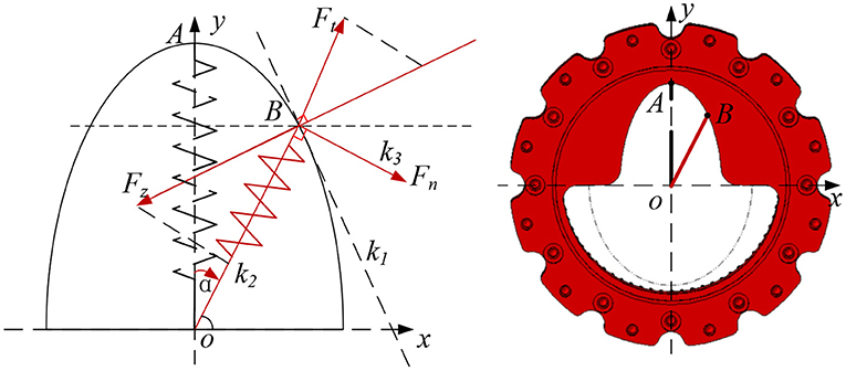When there is relative rotation between the input flange and the output flange, the gear 3 rotates, and the encoder collects the rotation degree of the magnetic steel to obtain the relative rotation angle between the two flanges, that is, the deformation angle.

In the variable stiffness joint with special curved surface, the design of cam contour determines the stiffness characteristics of the compliant joint, which needs to be analyzed and designed according to the contour. The variable stiffness joint designed in this paper is intended to be applied to the elbow rehabilitation robot. According to the existing literature research, the stiffness of the human elbow joint varies from 0 to 20 Nm/rad, and the output torque is 10 Nm. Therefore, the variable stiffness joint designed in this paper should meet the above index requirements.

Here, for the convenience of analysis, the output flange in Figure 3A is fixed, and the cam follower is idealized as a point. As shown in Figure 4, the cam contour is designed as an ellipse, the center of the cam disc is the o origin, the long axis of the cam contour is in the positive direction of the y axis, and the short axis is in the positive direction of the x axis. The xoy coordinate system is established.

Figure 4. Theoretical analysis of special surface.

Assuming that the length of the short axis of the ellipse is a and the length of the long axis of the ellipse is b, combined with Figure 4, the general equation of the elliptic curve is parameterized:

,,,]},,,]},,,]},,,,,]}],"socialLinks":[,"type":"Link","color":"Grey","icon":"Facebook","size":"Medium","hiddenText":true},,"type":"Link","color":"Grey","icon":"Twitter","size":"Medium","hiddenText":true},,"type":"Link","color":"Grey","icon":"LinkedIn","size":"Medium","hiddenText":true},,"type":"Link","color":"Grey","icon":"Instagram","size":"Medium","hiddenText":true}],"copyright":"Frontiers Media S.A. All rights reserved","termsAndConditionsUrl":"https://www.frontiersin.org/legal/terms-and-conditions","privacyPolicyUrl":"https://www.frontiersin.org/legal/privacy-policy"}'>