This study was approved by the Temple University Institutional Review Board (protocol #25913) and the Ministry of Health of the Kingdom of Saudi Arabia (protocol # H-05-FT-083). The convenience sample consisted of 23 young adults, 14 females and 9 males, with a previous diagnosis of vestibular migraine (average age 34.74 ± 8 years) who presented to the outpatient Otoneurology and Emergency Departments at Hafer Al-Batin Central hospital between the period of December 2020 and February 2021. Data from the healthy participants have been previously reported [26].

Those willing to participate provided informed consent. Of those, 13 participants with vestibular migraine tested positive for VVM (+ VVM) and 10 tested negative for VVM (−VVM) on the Visual-Vestibular Mismatch Questionnaire (Table 1) [32]. In a separate visit, vestibulonystagmography (bi-thermal caloric, positional nystagmus, smooth pursuit, random saccade, gaze stability, optokinetic nystagmus, and oculomotor testing) was performed on all participants who experienced migraine. Values of the abnormal caloric testing result were established by the clinical laboratory as a directional preponderance of 25% or greater.

Participants stood on the center of a standard AIREX 20" × 16.4" × 2" balance pad (Advanced Medical Technology Inc., Watertown, MA) with their arms at their sides and their feet about shoulder-width apart. Participants were asked to maintain an upright standing position with their eyes open while wearing a head mounted display (HMD) and watching a virtual visual scene for 3 min. Each exposure to the dynamic visual environment was followed by a rest period of at least one min until any emerging symptoms of dizziness, nausea, or any discomfort were verbally reported as resolved. During the rest period, participants were seated and the HMD removed.

Participants were exposed to a three-dimensional complex visual environment generated by the software PosturoVR 0.8.3 (Virtualis, France) projected on the Oculus Rift HMD (Oculus Rift, CA). The field of view (FOV) of this device is more than 90 deg horizontal (110 deg on the diagonal). Vision of the real world is completely blocked, thereby providing a strong sense of immersion.

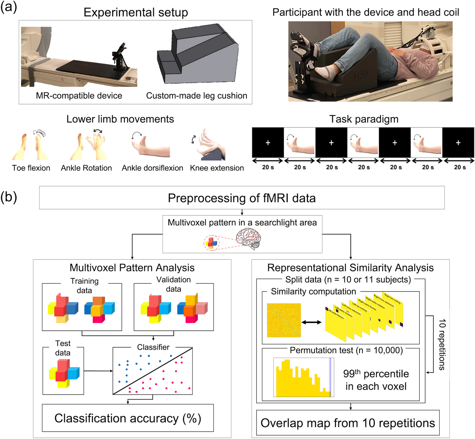
Two virtual environments (a space scene [SPACE] and a pedestrian crossing scene [STREET]) were randomly presented in one visit (Fig. 1). The space scene was a projection of star-like objects, at different sizes and distances from the participant, that rotated in the yaw axis with no cues indicating verticality. This image has been previously demonstrated to induce strong sensations of self-motion during quiet stance [33,34,35]. The direction of motion was in the direction identified by each participant as their dominant hand. The street crossing scene was constructed of three-dimensional, recognizable objects (i.e., buildings, sidewalks, traffic signals, cars, pedestrians) that moved in multiple directions at varied distances from the participant.

Images of the space (left) and street (right) virtual scenes

EDA is a measure of skin conductance and consists of a tonic component, also known as skin conductance level (SCL), which changes slowly over time (baseline) and reveals the active state of the sympathetic nervous system. A phasic component of the EDA, known as the skin conductance response (SCR), changes rapidly in response to external new, unexpected, and/or arousal-driven stimuli [17]. Sudden shifts of phasic activity above the tonic activity designate the SCR peaks.

Changes in EDA were recorded using the wireless Shimmer3 GSR + sensor unit (Shimmer-North America, Cambridge MA) that measures changes in skin conductivity produced by increases in the activity of sweat glands at a sampling rate of 128 Hz. The sensor was placed over the palmar surface of the medial metacarpal-phalanges of the third and fourth fingers of the non-dominant hand. Participants were instructed to close their eyes and relax until the investigator observed that activity detected and displayed by the Shimmer sensor unit remained close to a baseline.

Trunk triaxial linear acceleration data were tracked with a Shimmer3 IMU wearable sensor with a sampling rate of 128 Hz placed over the L5 vertebral region.

The presence of VVM, dizziness, balance confidence, and the level of physical activity of each individual were evaluated at the beginning of the experiment using validated clinical tools. The Visual-Vestibular Mismatch Questionnaire (VVMQ) [32] presents situational questions to determine the presence of the cluster of symptoms that define VVM. The Visual Vertigo Analog Scale (VVAS) [36] ranks the intensity of dizziness in environments with dynamic visual input. The Dizziness Handicap Inventory (DHI) [37] quantifies the self-perceived impact of dizziness on activities of daily life. The Vertigo Symptoms Scale-Short Form (VSS-SF) [38] uses a five-point Likert scale to determine the frequency of symptoms. The Activities of Balance Confidence (ABC) scale [39] is a self-reported measure of balance confidence during various motor activities. The Rapid Assessment of Physical Activity [40] assesses the daily level of physical activity. Combined, these scales provide a general overview of whether dizziness and instability are affecting quality of life and daily functional activity.

The presence of visual dependency was confirmed with a Rod and Frame test (RFT) available on the PosturoVR 0.8.3 software (Virtualis, France) and projected on to the Oculus Rift [8]. At the beginning of each trial, the virtual rod was set randomly at a 45 deg angle to the left or right. The rod was then rotated manually (1 deg/button press) by the investigator toward a vertical position. Participants were instructed to raise their hand to signal when they perceived that the rod had achieved a vertical position. Throughout these trials, the contextual square frame was tilted 28 deg to the left. The same procedure was repeated four times and the measure of angular deviation from vertical averaged for later analysis.

Raw EDA data was processed with MATLAB R2020b (The MathWorks, Inc., Natick, Massachusetts, USA) using the Ledalab-toolbox V3.4.9 (www.ledalab.de) through continuous decomposition analysis (CDA) to decompose the skin conductance data into its phasic (SCR) and tonic (SCL) components [41]. The CDA method can be applied to full-length data which provides a complete decomposition model of the original data. All mathematical models of CDA are based on a physiological rationale to avoid underestimation biases due to overlapping responses. However, the integrated skin conductance response (ISCR), defined as the area (time integral) of the phasic component within the response window, reflects the phasic EDA response to a given event or stimulus. It equals SCR multiplied by the size of the response window [Microsiemens (\(\mathrm)*\mathrm(\mathrm\))]. The detection threshold for significant peaks was set to 0.01 \(\mathrm\) as recommended by the Society for Psychophysiological Research [18]. To prevent the common skewed distribution of electrodermal response measures, the standardized ISCR was computed as [41]:

$$ISCR=log(1+|ISCR|)\times sign(ISCR)$$

Trunk linear acceleration data was processed using MATLAB R2020b (The MathWorks, Inc., Natick, Massachusetts, USA) which provides a formula for calculating the Root Mean Square (RMS) and the Normalized Path Length (NPL). RMS and NPL were calculated for the antero-posterior (AP), medio-lateral (ML), and vertical (VERT) planes where a higher values indicate greater postural instability [42,43,44,45]. RMS is the mean power of the entire trial time and NPL is the sum of the absolute values of acceleration over time divided by the length of time that it takes to travel that distance, thus describing smoothness of the trunk motion. RMS and NPL were computed using the following formulae [45]:

$$RMS=\sqrt\frac^_}\end\right)}^\end} NPL=\frac\sum_^|_-_|$$

where \(t\) is time duration, \(N\) is the number of time samples, and \(_\) is the acceleration data at time sample \(j\). Data were low-pass filtered using a 4th order Butterworth filter with a cutoff frequency of 1.25 Hz. Each trial was plotted individually and inspected visually to ensure that the data were free from significant artifacts.

EDA and six postural acceleration measures (RMS and NPL each in ML, AP, and VERT axes) were analyzed using R version 4.0.4 (R Foundation for Statistical Computing, Vienna, Austria). Correlations for continuous variables were computed with Pearson correlation coefficients with a two-tailed test. A Shapiro–Wilk test revealed the data were normally distributed.

Linear mixed-effect (LME) models were constructed to statistically assess the effects of the virtual visual environments (SPACE and STREET) across groups (+ VVM and −VVM) and time. Response variables included ISCR, NPL, and RMS with the subject as a random effect and a slope fit for each trial. LME models were fit using restricted maximum likelihood estimation [46]. After examining the full-effects model for EDA phasic, EDA tonic, RMS, and NPL responses in the AP, ML, and VERT planes, non-significant terms and interactions were removed. The final model for estimating the change in EDA phasic response included the interaction of group with time.

Specific differences between the virtual environments and groups were examined with a Wilcoxon signed rank test. Effect sizes were calculated using the following formula [47]:

$$\mathrm=\mathrm/\surd \mathrm$$

where \(r\) is the effect size, \(Z\) is the Z statistic, \(N\) is the sample size. Effect sizes were classified as follows: no effect (0.0 to < 0.1); small effect (0.1 to < 0.3); medium effect (0.3 to < 0.5); and large effect (≥ 0.5) [47]. For t-tests, the usual Cohen's d effect size measure was computed [47].

Data from self-reported outcome measures were analyzed using IBM SPSS Statistics v.23 (IBM Corporation, Armonk, N.Y., USA) and reported as mean ± standard deviation or as a percentage of participants. The significance level was set at α = 0.05 for all analyses. Bonferroni post-hoc adjustments were used to adjust for multiple comparisons. Differences in demographics and clinical outcome scores between the + VVM and −VVM groups were assessed using Welch’s t-test. Individuals were assigned positive or negative results on the RFT based on the criterion of an angle of deviation greater than 5 deg to indicate visual dependency [8].