Aquaculture is one of the fastest-growing food production industries, with an annual production of 130.9 million tons and a value of approximately 312.8 billion USD, while also maintaining a lower carbon footprint compared to terrestrial animals (Norman et al., 2019; FAO, 2024). Mussels are considered one of the major bivalve species cultured worldwide, with France ranking as the second largest European producer, producing 71,311 tons in 2022 (FAO, 2024). Two species as well as their hybrids are cultivated in France: the blue mussel Mytilus edulis, and the Mediterranean mussel Mytilus galloprovincialis. Production is distributed along the English Channel to the southwest coastline of France, and Mediterranean shores (Prou and Goulletquer, 2002). Mytilus species has been widely cultured due to its strong environmental adaptability, high nutritious value, and consumer preference (Prou and Goulletquer, 2002; Suplicy, 2020). French mussel production entirely relies on wild spat collection, mainly in Pays de Loire and in Nouvelle-Aquitaine regions (Prou and Goulletquer, 2002). Consequently, the French cultivated mussels are not genetically selected through selective breeding programs.

Massive mortality outbreaks have been reported in various bivalves species including mussels worldwide, significantly impacting production, causing economic losses, and negatively affecting ecosystems, with the cause often remaining unidentified (Degremont et al., 2007; Bódis et al., 2014; Burdon et al., 2014; Soon and Ransangan, 2019; Capelle et al., 2021; Lupo et al., 2021; Ericson et al., 2023). Since 2014, abnormal mussel mortality (AMM) outbreaks have been reported in French mussel farms, with mortality rates ranging from 10% to 99% depending on sites, seasons or years with peak mortality observed in the springs of 2014, 2016, and 2018 (Polsenaere et al., 2017; Degremont et al., 2019; Normand et al., 2022). Previous studies have identified several factors linked to AMM outbreaks, including seawater characteristics, pollution, mussel characteristics, culture practices, pathogens and climate change (review by Lupo et al., 2021). Various strains of Vibrio splendidus isolated from moribund mussels at sites affected by mass mortality have been linked to the AMM outbreaks (Bechemin et al., 2015; Ben Cheikh et al., 2016). Vibrio splendidus is a complex species comprising multiple strains, ranging from highly virulent to relatively innocuous (Ben Cheikh et al., 2016). Some virulent strains have been shown to be highly pathogenic to blue mussels, causing high mortality rates up to 90% within a week in experimental challenges (Ben Cheikh et al., 2016; Oden et al., 2016; Ben Cheikh et al., 2017). The virulence of these strains can vary based on several factors including mussel characteristics, environmental conditions, and seasons (Charles et al., 2020). While V. splendidus is not the direct cause of AMM, its consistent association with mortality outbreaks suggests it may play a contributory role under specific conditions. Recent studies on bivalve immune responses often lack a validated understanding of immune effectors or pathways, reflecting their reliance on innate rather than adaptive immunity, limiting the efficacy of vaccination strategies (Allam and Raftos, 2015; Rey-Campos et al., 2019). Selective breeding could be a useful approach to enhance the innate immune responses in bivalves (Degremont et al., 2015; Hollenbeck and Johnston, 2018). Understanding genetic basis of disease resistance is critical for its improvement through selective breeding.

Over the past decades, many commercially important bivalve species have demonstrated significant genetic improvement through mass selection, due to their high fecundity and short generation intervals (Gjedrem and Rye, 2018; Tan et al., 2020). Mass selection has been carried for growth traits in Chilean blue mussel Mytilus chilensis (Toro et al., 2004a; Toro et al., 2004b), and ploidy status for Mediterranean mussel M. galloprovincialis (Ajithkumar et al., 2025). Lately, a mass selection scheme implemented for resistance to AMM outbreaks in the blue mussel M. edulis resulted in a 34%–48% increase in survival after one generation of selection (Degremont et al., 2019). Although mass selection is effective, it may quickly lead to inbreeding if genetic diversity is not properly monitored (Hu et al., 2022). However, family based selective breeding programs have been initiated as an alternative strategy to mass selection, to estimate breeding values by combining phenotypic information and pedigree. These programs have targeted various traits across different mussel species, such as growth in M. edulis (Mallet et al., 1986), M. galloprovincialis (Nguyen et al., 2014; Pino-Querido et al., 2015; Díaz-Puente et al., 2020), M. chilensis (Alcapán et al., 2007; Guiñez et al., 2017), Hyriopsis cumingii (Jin et al., 2012; Bai et al., 2017), Perna calaniculus (Camara and Symonds, 2014); shell nacre color in H. cumingii (Bai et al., 2017); toxin accumulation and mantle color in M. galloprovincialis (Pino-Querido et al., 2015); and survival in M. edulis (Mallet et al., 1986).

Accurate estimations of breeding values are crucial for developing a successful breeding program and predicting the responses of traits of interest to selection. Advances in high-throughput genotyping technology have now made it possible to implement genomic selection effectively in aquaculture species (Boudry et al., 2021). Genomic selection is especially beneficial for traits that are costly or difficult to measure, such as flesh quality or disease resistance, and it can achieve similar or higher accuracies in estimated breeding values (EBVs) with less phenotypic data compared to traditional family-based selection (Regan et al., 2021; Yáñez et al., 2023). Furthermore, genomic selection enhances genetic gain by capturing genetic variation both within and between families (Boudry et al., 2021). Next-generation sequencing and genotyping-by-sequencing tools have been developed to detect genome-wide molecular markers for oyster, clam, abalone and scallop (Jiao et al., 2014; Ren et al., 2016; Wang et al., 2016; Nie et al., 2017; McCarty et al., 2022; Yang et al., 2022). However, these methods may not provide reliable markers for testing across different populations (e.g., between the training and breeding populations) because they sequence a large number of randomly distributed regions, and their effectiveness can vary with DNA quality, limiting their ability to produce consistent genomic analyses (Davey et al., 2011; Boudry et al., 2021). Alternatively, SNP arrays have been developed for several commercially important bivalve species, including silver-lipped pearl oyster (Pinctada maxima), with an Illumina ∼3k iSelect custom array (Jones et al., 2013a), the medium density bi-species (Pacific oyster Crassostrea gigas and European flat oyster Ostrea edulis) 57K SNP array (Gutierrez et al., 2017), the Pacific oyster (C. gigas), with a 190K SNP array (Qi et al., 2017), the Eastern Oyster (C. virginica), with a high density 566K and 66K SNP array (Guo et al., 2023), or medium density multi-species (M. edulis, M. galloprovincialis, M. trossulus, and M. chilensis) 60K SNP array (Nascimento-Schulze et al., 2023), all of which rely on commercial chip products with fixed sets of markers and specific genotyping platforms. SNP arrays have been applied to a range of aquaculture species for various purposes, such as uncovering the genetic architecture of traits, implementing genomic selection, characterizing genetic resources, pedigree monitoring, sex-determination, and inbreeding management. However, their use in bivalves has been relatively limited (Gutierrez et al., 2020; Jourdan et al., 2023).

In aquaculture, the salmon industry has been leading the way in genomic selection for several years (Odegård et al., 2014; Tsai et al., 2015; Correa et al., 2017; Robledo et al., 2018; Ajasa et al., 2024). To date, more frequently aquaculture species are following this trend such as rainbow trout Oncorhynchus mykiss, European sea bass Dicentrarchus labrax, Gilthead Sea Bream Sparus aurata, Nile tilapia Oreochromis niloticus, Channel catfish Ictalurus punctatus or whiteleg shrimp Litopenaeus vannamei [see for review (Houston et al., 2020; Boudry et al., 2021; Song et al., 2022; Yáñez et al., 2023)]. The recent advancements in genotyping tools have paved the way for exploring the potential of genomic selection in bivalves. Genomic selection has been investigated in the Portuguese oyster for morphometric traits, edibility traits and disease traits (Vu et al., 2021), in the American oyster for low salinity tolerance (McCarty et al., 2022),in the silver-lipped oyster for pearl quality traits (Zenger et al., 2019) and growth traits has been studied in the triangle sail mussel (Wang et al., 2022), European flat oyster (Penaloza et al., 2022) and Pacific oyster (Gutierrez et al., 2018; Jourdan et al., 2023). A few studies have been conducted in oysters showing the increase in accuracy of genomic selection over pedigree-based approaches for difficult to measure traits, such as disease resistance, meat content and color traits (Gutierrez et al., 2018; Gutierrez et al., 2020; Jourdan et al., 2023). To date, trials with low-density panels to reduce genomic evaluation costs have been conducted in several aquaculture species, indicating that developing cost-effective strategies for genomic selection will be pivotal in shaping modern aquaculture breeding programs (Kriaridou et al., 2020; Penaloza et al., 2022).

The primary aim of our study was to evaluate the potential of genomic selection for resistance to one pathogenic strain of V. splendidus in M. edulis. Using a multi-species Axiom Affymetrix 60K SNP array (Nascimento-Schulze et al., 2023), we first characterized the genetic structure and linkage disequilibrium of the blue mussel population. We then estimated genetic parameters for resistance to V. splendidus and performed GWAS to investigate its genetic architecture. Finally, we compared genomic and pedigree-based selection accuracies to optimize breeding programs.

The 48 families of M. edulis used in this study are detailly described in (Ajithkumar et al., 2024b). Briefly, three wild mussel populations were sampled, two from the Atlantic coast (OLE-PON and YEU_001), and a third from the North of France (WIM), and transferred to the Ifremer hatchery in La Tremblade in the fall of 2016. Each mussel population was cleaned and placed in separate tanks containing unheated UV-treated, and filtered seawater (400 L per hour). To favor gametogenesis, mussels were fed a cultured phytoplankton diet (Isochrysis galbana, Tetraselmis suecica, and Skeletonema costatum). Two sets of crosses were performed in January 2017 (set 1) and in February 2017 (set 2). For each population, 100 mussels were individually placed in 400 mL beakers, and spawning was triggered by alternating cold (10°C) and warm seawater (20°C). Depending on the ripeness of the mussels and the sex ratio, four males for OLE-PON, and 11 males for YEU_001 were used in set 1, while 9 males were used for WIM in set 2. Within population, each male was mated with two females, producing in total 24 half-sib families, each containing two full-sib families. These 48 full-sib families consist of 8, 22 and 18 families from OLE-PON, YEU_001 and WIM population, respectively, all should be considered as outbred. Each full-sib family was grown separately in 30 L tanks filled with filtered and UV-treated seawater at 20°C until the pediveliger stage. Then, downwelling system were used until mussels reached 1 cm. At that size, they were transferred to our nursery in Bouin in April and May 2017 for set 1 and set 2, respectively. For each family, 1,000 spat were maintained in 15 L SEAPA© baskets, and all families were raised in a 20 m³ concrete raceway until the start of the experiment, which occurred in July 2018. More detailed on the larval and nursery culture are provided in Ajithkumar et al. (2024b).

Detailed step-by-step protocol of the experimental infection is given in Ajithkumar et al. (2024b). Briefly, two experimental infections (EI_1 and EI_2) were conducted in July 2018. Among the 48 families (mean individual total weight of approximately 5 g), 24 families were randomly sampled and tested in El_1, and the others were tested in El_2. Additionally, a third experimental infection (EI_3) was performed, involving the same 24 families from El_1, to increase the genotype sample size due to some samples from El_1 were lost. Finally, three families tested in El_2 were also tested in El_1, leading to a total of 27 families tested in El_1, and one of those three was also tested in El_3 indicating that only one family was tested in each of the three experimental infections (see Supplementary Table S1 for details). For each experimental infection and family, a highly pathogenic strain of V. splendidus (strain 14/053 2T1) isolated during AMM outbreak in 2014 was injected in 30 mussels to investigate their resistance to this pathogen. This particular strain was selected for its high virulence, the highest among the 50 strains tested, and it belongs to a specific pathogenic group. The lethal dose-50 (LD50) was determined prior to the experimental infection by injecting varying concentrations of Vibrio splendidus strain into a large group of mussels. The selected dose was close to the LD50, ensuring adequate variance in the response for effective assessment of resistance. First, mussels were anesthetized using MgCl2 (50 g per L), and 50 μL of bacterial solution (109 bacteria/mL) was injected into the muscle. Then, ten injected mussels per family, for all the 24 families of one set were hold in one 120 L tank containing UV-filtered seawater. Three replicate tanks were used and, in each tank, water recirculation was maintained using a TECO®pump (Ravenna, Italy), which also maintained the seawater temperature at 17°C. Dead mussels were counted and sampled daily up to 72 h post-injection. The adductor muscle/gills of the dead mussels during the experiment and the surviving mussels at the end of the experiment were collected using scalpels disinfected with 70% ethanol and stored in 1.5 mL sterile tubes at room temperature.

Among the dead and alive animal sampled, around 14–15 mussels were genotyped per family (ranging from 13 to 16) (Table 1; Supplementary Table S1). The number of dead and alive per family was calculated in proportion to the mortality observed within each family in El_1 and in El_2. As the number of animals sampled in El_1 was not sufficient, 158 dead mussels and 35 live mussels were sampled from EI_3 (Supplementary Table S1). In total, 768 individuals were genotyped; 348 dead, 348 alive, and the remaining 72 were their parents (48 dams and 24 sires). DNA extraction and genotyping were performed by the Gentyane INRAE Platform (Clermont-Ferrand, France) using the multi species medium-density 60K SNP-array, Axiom_Myt_v1_r1 (Thermo Fisher Scientific, Waltham, Massachusetts, United States), which comprises 23,252 markers for M. edulis (Nascimento-Schulze et al., 2023). Quality controls on the 60K SNPs from the SNP array and genotyped individuals were performed as described in D'Ambrosio et al. (2019). Firstly, genotypes of all individuals were analyzed using the Axiom Analysis Suite software (AxAS; v.4.0.3.3) with the default best practice workflow suggested by the manufacturer, with few threshold modifications, which includes individual quality control and SNP quality control analysis (Dish Quality Control ≥0.20; Quality Control call rate ≥90; percent of passing samples ≥98; average call rate for passing samples ≥92%; call rate cutoff ≥95; Fisher’s Linear Discriminant ≥2.6). Consequently, 7,476 polymorphic SNPs were retained for further analysis. Subsequently, final quality control was performed using PLINK v1.9 software (Chang et al., 2015). Two individuals with an identity-by-descent value over 0.90 were considered as duplicated and both individuals were removed from the analysis. Only SNPs with a minor allele frequency (MAF) higher than 0.01 and those passing the Hardy-Weinberg equilibrium test (p-value <0.0000001) in the genotyped mussels were retained. After the quality control, data comprised of a total of 766 genotyped individuals for 3,406 SNPs.

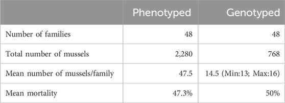
Table 1. Summary of the experimental infection using the pathogenic strain 14/053 2T1 of Vibrio splendidus in Mytilus edulis.

Parentage assignment was performed in the R package APIS (Griot et al., 2020) with a mismatch number set to 5%. The best 1,471 SNPs, selected with call rate greater than 90% and MAF value greater than 0.1 were used. Parentage assignment allowed the reconstruction of the pedigree of 647 offspring with assignment rates reaching 93.2% of the mussels having both parents assigned, while the remaining 47 mussels potentially from outside the cross-mating design, which were excluded from following analyses.

To evaluate potential genetic sub-structuring of populations and any associated biases, a principal component analysis (PCA) was performed using PLINK 1.9 (Chang et al., 2015) and the genetic structure was visualized using in RStudio (Team, 2024). Three individuals were identified as outliers beyond the population structure and were subsequently excluded from further analysis. Genetic differentiation between populations was measured through pairwise fixation index (FST) estimates using PLINK 1.9 (Chang et al., 2015).

All markers of the array along with their flanking regions were blasted using a BLASTn® procedure on the reference genome (Mytilus edulis genome assembly, xbMytEdul2, GenBank accession number: GCA_963676595.2). To map SNPs, considering the high polymorphism in the mussel genome, four mismatches were allowed over a length of around 71 base pairs. Only SNPs mapping to a unique position on the reference genome were retained for the subsequent stage of quality control as mentioned in previous section. Out of the 3,406 SNPs, only 2,204 matched our mapping criteria and were successfully positioned on the reference genome (Supplementary Table S2).

The pairwise linkage disequilibrium (LD) analysis was performed between all SNPs and adjacent markers for each linkage group and population to determine LD decay within the genome of M. edulis using Plink 1.9 (Chang et al., 2015).

Estimated breeding values, variance components, and heritability were calculated using the BLUPF90 software package (Misztal et al., 2014) through two different approaches: a linear mixed model with AIREMLF90 (Misztal et al., 2014) for assessing the trait on the observed scale, and a Gibbs analyses with THRGIBBS1F90 (Tsuruta and Misztal, 2006) for evaluating it on the underlying scale, based on pedigree-based relationship.

where Y is the binary mortality outcome at the end of the experiment (1 = dead, 2 = alive) of mussel, β is the vector of fixed effects, including set of crosses (set 1, set 2), population origins (OLE-PON, WIM, YEU_001), and replication of the experimental infection (EI_1, EI_2 and EI_3). μi is the vector of additive genetic effect of the animal, following a normal distribution μ ∼ N0,Aσa2, where A is the pedigree relationship matrix, and σa2 is the additive genetic variance. e is the vector of random residuals, assumed to be distributed as e∼N(0,Iσe2 where I is an identity matrix and σe2 is the residual variance. X and Z are known incidence matrices relating observations to the fixed and random effects mentioned above. Random tank effect was removed from the model due to the lack of significance.

The EBV were estimated using BLUPF90 package and the variance components using AIREMLF90 and THRGIBBS1F90 programs. With the threshold model, the variance components were estimated using a Gibbs sampler with 100,000 iterations, 10,000 of burn-in and one sample was kept every 10 iterations for posterior analysis. Variance components were estimated using the average information restricted maximum likelihood algorithm (Gilmour et al., 1995). The h2 for linear model on observed scale transferred into underlying scale using the formulae from Dempster and linear (1950).

Heritability (h2) was estimated as: h2=σa2σa2+σe2

Estimated heritability was calculated using animal linear model with AIREMLF90 and animal threshold model with Gibbs sampling using THRGIBBS1F90. The GBLUP model uses the same approach as the PBLUP model, but A replaced by G. Here, G is the genomic relationship matrix. The matrix G was computed as described by VanRaden (2008).

where Z is a matrix of centered genotypes 0−2p= homozygous, 1−2p= heterozygous, 2−2p= homozygous), pi is the frequency of the reference allele for the ith marker, and m is the total number of markers.

The population-specific analysis was performed using SNP markers to estimate heritability within population, and genetic correlation between populations. A high genetic correlation (0.99) was observed between populations (Supplementary Table S3).

Estimated heritability was calculated using animal linear model with AIREMLF90 and animal threshold model with Gibbs sampling using THRGIBBS1F90. The single-step GBLUP (ssGBLUP) model enhances the PBLUP and GBLUP model by fitting the H matrix, which integrates both genomic and pedigree data (Aguilar et al., 2010). The inverse of the H matrix was constructed as follows:

where G is as described above and A22 is the pedigree-based relationship matrix for genotyped animals.

To identify SNPs associated with resistance to V. splendidus, a genome wide association study (GWAS) was performed using a mixed linear model association through ssGBLUP analysis. The postGSF90 module (Misztal et al., 2014) from the BLUPF90 package was used to estimate the effects of the SNPs (a^i) based on the genomic breeding values g^i predicted for the genotyped animals. The SNP effects were estimated according to the following equation:

where d is the vector of weights associated with the SNP effects and Z is the incidence matrix relating SNP effects to genomic breeding values.

Estimates of SNP effects (a^i) can be used to estimate the proportion of additive genetic variance of each SNP effect:

with σa2 the total genetic variance estimated using the linear mixed model with postGSF90 and p the minor allele frequency of the target SNP.

Prediction accuracy for the PBLUP, GBLUP, and ssGBLUP models was assessed using the ‘leave-one-out’ method, implemented with a linear model in BLUPF90 (Resende et al., 2012; Kristensen et al., 2018). In this approach, each observation is systematically excluded one at a time. The model is then trained on the remaining data, and the (G)EBV for the excluded individual is predicted by masking its phenotype.

The accuracy (r) of prediction was computed as the correlation between the (G) EBVs and the corrected phenotype (y^) of the mussel divided by the square root of the heritability, using the formula:

The heritability value h2 used in this analysis was calculated using the variance components (σa2 and σe2 from the ssGBLUP model.

The cumulative mortality rate 72 h post-injection was 47%. At endpoint, mortality rates were 63% for EI_1, 41% for EI_2, and 37% for EI_3. Among mussel populations, the WIM population (54%) showed higher susceptibility to V. splendidus compared to the YEU_001 (45%) and OLE-PON (37%) populations (Supplementary Table S4). Mortality rates varied significantly among families upon exposure to V. splendidus, ranging from 17% to 83%. The mean mortality rates for all families are depicted in Figure 1.

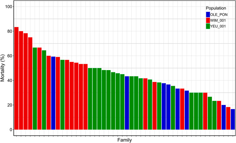
Figure 1. Final cumulative mortality 72 h post-injection for each family. Each bar represents a family and each color represent a population.

Figure 2 illustrates the results of the principal component analysis (PCA), revealing the population structure of the mussel population. The first two PCA axes collectively account for over 15% of the total genetic variation. The YEU_001 and OLE-PON populations were generally homogeneous, although there were few stratifications within YEU_001. The WIM population have quite different genetic background from others, with two families whose offspring showed even greater isolation. Nevertheless, FST analysis revealed low genetic differentiation between populations. The mean genetic distances between populations are shown in Table 2, with FST values ranging from 0.02 to 0.03, suggesting genetic similarity across all three populations (Figure 3).

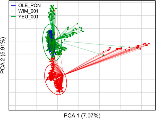
Figure 2. First two axes and associated variances of the principal component analysis (PCA) of the genetic diversity among the three populations of Mytilus edulis. The ellipses are constructed with axes defined as 1.5 times the standard deviation of the projections of individual coordinates on the axes. PCA was performed with 647 individuals and 3,406 SNPs.

Table 2. Pairwise FST between populations of Mytilus edulis.

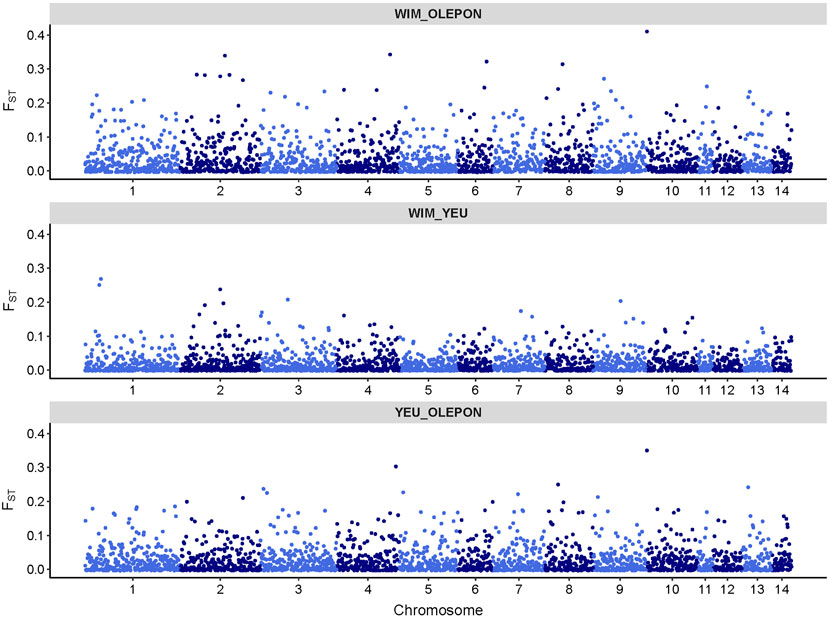
Figure 3. Genomic distribution of fixation index (FST) values as a function of chromosome position in the mussel genome for different studied population.

2,204 SNPs were positioned on the reference genome, resulting a loss of 1,202 SNPs. The positions of markers on the chromosomes are illustrated in Supplementary Figure S1. The average SNP density per megabase (Mb) ranges from 0.57 to 2.37, varying among chromosomes and within chromosome (Supplementary Table S5). Approximately, only 9% of all 1 Mb segments contain more than 5 SNPs. SNP density exhibits non-uniformity throughout the genome, with each chromosome demonstrating varying densities. The lower marker density results in greater mean average distances between adjacent SNPs, ranged from 421 kb to 1739 kb depending on the chromosome.

Figure 4 illustrates that linkage disequilibrium (LD) decreases sharply as the distance between pairs of SNPs increases, with the most rapid decline occurring within the first 100 kb. Beyond this range, LD continues to decline and becomes more variable. The OLE-PON population consistently shows higher LD throughout the genome compared to other populations. On average, the LD values (r2) for SNPs less than 15 kb apart are 0.12 for OLE-PON, 0.10 for WIM, and 0.06 for YEU. Linkage disequilibrium values are generally low between adjacent SNPs for all the chromosomes, where distances between adjacent SNPs are larger.

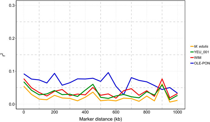
Figure 4. Linkage disequilibrium (r2) decay with physical distance between markers in each population and overall challenged to Vibrio splendidus. The X-axis is the physical location, and the Y-axis is the linkage disequilibrium value (r2).

The estimates of heritability using the linear and Gibbs sampling models are summarized in Table 3. Pedigree-based heritability estimates for resistance to V. splendidus in M. edulis ranged from 0.22 to 0.31. Genomic heritability was slightly higher, varying between 0.33 and 0.36. The ssGBLUP based estimated heritability ranging from 0.28 to 0.33, which combines genomic and pedigree information.

Table 3. Heritability for resistance to Vibrio splendidus in Mytilus edulis.

GWAS for resistance to V. splendidus suggest that this trait is likely to be impacted by multiple genomic regions. However, there were 20 SNPs that explained >0.5% of additive genetic variance on chr 1, chr 2, chr 3, chr 4, chr 5, chr 6, chr 8, chr 9, chr 13, and chr 14 (Figure 5). However, none of these markers explained more than 1.06% of the additive genetic variance (Figure 5; Table 4).

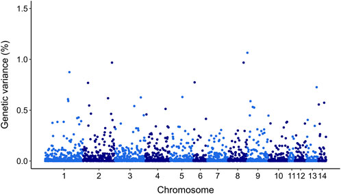
Figure 5. Manhattan plot of genetic variance explained by each SNP for resistance to Vibrio splendidus in Mytilus edulis using ssGBLUP approach. In X-axis SNP per chromosome and Y-axis percentage of genetic variance explained per each SNP.

Table 4. Summary of top five SNPs associated with resistance to Vibrio splendidus in GWAS analysis (ssGBLUP) ranked with respect to genetic variance. Position = Physical position of SNP on the chromosome; A1 and A2 = Minor and major alleles, respectively; MAF = Minor allele frequency; var A = percentage of additive genetic variance explained by SNP.

Accuracy with all data are 0.36, 0.43, 0.43 for PBLUP, GBLUP and ssGBLUP, respectively. Genomic selection (GBLUP and ssGBLUP) is better than PBLUP by 19%. Overall, prediction accuracy for genomic selection increased with the density of markers (Figure 6). Incorporating genomic information generally enhanced accuracy compared to pedigree-based estimation, except with 500 SNPs where PBLUP exhibited higher accuracy than GBLUP (Figure 6). With maximum training population and SNP subsets, genomic evaluation improved accuracy by 17%, 19%, 25%, and 19% for 1,000, 1,500, annotated (2,204), and all SNPs (3,406), respectively, compared to PBLUP. When comparing GBLUP and ssGBLUP models, the prediction accuracy was consistently favored the ssGBLUP model, except when using annotated SNPs in the GBLUP model (Figure 6).

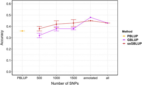
Figure 6. The estimated prediction accuracy of Vibrio splendidus resistance in Mytilus edulis using PBLUP, GBLUP and ssGBLUP across different marker densities. Each point is the average of 5 replicates. Error bars represent the standard error of the mean of 5 replicates. PBLUP - Pedigree based breeding values using all phenotyped animals, respectively. GBLUP - Genomic breeding values from only genotype animals, and ssGBLUP - Genomic breeding values from all genotyped and phenotyped animals obtained with a combined relationship matrix (H). Annotated: SNPs mapped onto the recently published reference genome (2,204); all: retained SNPs after quality control (3,406).

In our study, we aimed to demonstrate the feasibility of genomic selection in a mussel breeding program in France. We used a recently developed multi species medium-density 60K SNP-array (Nascimento-Schulze et al., 2023) to perform genomic analysis. Combining multiple populations is a common approach for multi-population GP and combined GWAS analysis (VanRaden et al., 2009; Lund et al., 2011; Begum et al., 2012). However, there are three criteria for using this approach: first, the trait of interest is measured in the same way in different populations and genotyping is done using same SNP array; second, there is no G × E interaction in different populations; and finally, the genetic distance between the populations is minimal (Lund et al., 2011; Begum et al., 2012; Gebreyesus et al., 2019). As our study meets these requirements, combined population analyses were performed.

To the best of our knowledge, our study is the first to use the multi species medium-density 60K SNP-array (Nascimento-Schulze et al., 2023) to estimate genetic and genomic parameters in blue mussel (M. edulis). After all quality controls, we identified high-quality SNPs from 23,252 SNPs present on the array across 768 individuals. The necessity for stringent filtering of genotyping data is highlighted by the prevalence of poor-quality markers. One of the distinguishing features of the Mytilus species complex is its high degree of heterozygosity and abundance of mobile elements, which pose challenges in accurately identifying polymorphic SNPs (Gerdol et al., 2020; Sun et al., 2017). Compounding this difficulty, the current SNP array was developed using a whole-genome low coverage approach, which can lead to loss of polymorphic sites, especially across genetically diverse populations. A prior study validating this SNP array found 89.8% of the 23,252 SNPs to be polymorphic due to the close genetic match between the populations used for development and validation (Nascimento-Schulze et al., 2023). In contrast, after quality control in our study, only 14.6% of the SNPs were retained as polymorphic, likely due to genetic differences between our sampled population and the one used for array creation. This discrepancy highlights the influence of population structure on SNP retention and substantial genetic complexity and high polymorphism exhibited in mussel genome (Gerdol et al., 2020; Smietanka et al., 2014). This complexity stems from its evolutionary history of extensive gene flow among related species and a genome characterized by significant dispensable content. Indeed, about 30% of genes in Mytilus are dispensable, likely impacting SNP distribution and usability across populations (Gerdol et al., 2020). Out of 23,252 SNPs identified in M. edulis, without any other quality control, only 16,213 (70%) were annotated on the recently published reference genome of M. edulis. Assembly errors in the reference genome may rise from several factors, such as exceptionally high genetic polymorphism levels, non-Mendelian segregation of marker loci in paired crosses, and a significant occurrence of null alleles in genetic markers (Hedgecock et al., 2015). If we consider the other quality controls done, only 2,204 SNPs (64.8% of polymorphic, good quality SNPs, 9.4% of the total available SNPs) mapping successfully. This limited SNP coverage and sparse distribution across the linkage map could potentially lead to the omission of QTLs in specific regions, particularly in regions where markers are underrepresented. To improve SNP array quality and increase the number of informative SNPs, future work could include strategies such as pooled sequencing with a greater number of individuals, incorporating genetically diverse populations, or performing high-coverage whole-genome resequencing numbers of individuals from each population (Nascimento-Schulze et al., 2023). These adjustments would increase the SNP array’s robustness, thereby improving genome coverage, QTL detection power, and marker-trait association accuracy in M. edulis.

The bi-species Axiom Affymetrix 57K SNP array has been used in Pacific oysters, where applying the AxAS software’s best practice workflow led to a notable reduction in the number of informative SNPs. Specifically, Gutierrez et al. (2018) reported 23,000 informative SNPs from 820 individuals, Vendrami et al. (2019) identified 21,499 SNPs from 232 individuals, and Jourdan et al. (2023) obtained 14,500 SNPs from 2,420 individuals. This reduction is largely attributed to the complex genetic structure of molluscs, stemming from the highly polymorphic nature of their genomes (Gerdol et al., 2020; Jiao et al., 2021; Song et al., 2021), and is further influenced by the genetic relationship between the training population used for array design and the breeding candidates in selective breeding program (Houston et al., 2020). However, recent studies on bivalves have demonstrated that a moderate number of high-quality markers (1,000–3,000) could suffice for accurate predictions (Gutierrez et al., 2018; Kriaridou et al., 2020; Penaloza et al., 2022).

Linkage disequilibrium (LD) at the genome level plays a crucial role in the efficacy of breeding programs, influencing genetic variance and the accuracy of association analyses (Goddard and Hayes, 2009; Siol et al., 2017). In our study, values for r2 ranged between 0.07 and 0.09 for SNPs within a distance of 10 kb and from 0.03 to 0.08 within 50 kb in the populations studied, suggesting limited short-range LD at current SNP marker densities. LD levels decreased to less than 0.05 at 100 kb in two populations. The high LD in OLE-PON is probably an overestimate due to a smaller effective population size (Ne) than in the other populations. Overall, LD between adjacent markers within each population was predominantly less than 0.1 within 2 kb, indicating a rapid decline in LD within the blue mussel genome. Therefore, these LD estimates should be treated with caution. This swift decay suggests a historically large effective population size and high recombination rate, reflecting substantial genetic diversity within the population (Ellegren and Galtier, 2016). Moreover, LD values are population-specific, and influenced by evolutionary factors such as natural selection, mutation, genetic drift, origin and migration, as well as molecular forces including historical recombination events, and breeding history such as historical effective population sizes, intensity and direction of artificial selection, population admixture, and mating patterns (Du et al., 2007). Our findings confirm the low LD in M. edulis populations, consistent with previous studies on bivalves (Jones et al., 2013b; Vera et al., 2022; Jourdan et al., 2023). However, the sparse SNP distribution and generally low LD values (r2 < 0.1) suggest that increasing marker density is essential to improve prediction accuracy and QTL detection.

FST is widely applied to evaluate genetic differentiation between/among populations (Hu et al., 2022). The low FST values (FST < 0.03) observed in our study suggest minimal genetic differentiation among mussel populations, indicating a lack of significant genetic structure. This phenomenon may be attributed to similar selection pressure and limited gene flow among the mussel populations, irrespective of geographic location. Similar to our findings, wild populations of M. edulis sampled from the Atlantic coast of France and from the Northern France to Germany had low Fst value (<0.003) using ancestry-informative SNPs (Simo