1 Introduction

Fear and stress drive adaptive behavior in response to environmental challenges. The activation of fear and stress responses triggers a cascade of autonomic and endocrine changes, significantly impacting learning and memory processes, as shown in seminal neurology and psychology research (Squire, 1987, 2009; McGaugh, 2013). The effects of these changes depend on their timing relative to the learning process (Drexler et al., 2019).

Pavlovian fear conditioning has become an essential tool for investigating cognitive paradigms in both human and animal research. This methodology has significantly enhanced our understanding of the physiological basis of fear and has applications in preclinical models of neuropathologies and clinical research (Chang et al., 2009). Through pre-training, post-training, and pre-test manipulations, Pavlovian fear conditioning provides insights into the complexities of memory acquisition, consolidation, and retrieval (LeDoux, 2000; Maren, 2011).

Fear conditioning involves associating a neutral stimulus or context with an unconditioned stimulus (US), resulting in the neutral stimulus acquiring aversive properties and becoming a conditioned stimulus (CS). This process elicits conditioned responses (CR), a well-documented phenomenon (Ehrlich et al., 2009). Additionally, extinction is introduced as a context-dependent learning form, describing the reduction of conditioned responses when the CS is presented without the US, leading to the suppression, but not erasure, of the memory (Turnock and Becker, 2008; Chang and Liang, 2017).

The efficacy of Pavlovian fear conditioning depends on the strength of the conditioned-unconditioned stimulus pairing and can be reversed during extinction processes. These limitations pose challenges in elucidating the mechanisms underlying stress and anxiety, affecting the development of effective behavioral therapies for related disorders (Maren et al., 2013; LeDoux, 2014; Maren and Holmes, 2016; Bennett et al., 2019). Consequently, stress models such as Immediate Extinction Deficit (IED) and Stress-Enhanced Fear Learning (SEFL) have been developed to understand stress's influence on fear memory.

The Stress-Enhanced Fear Learning (SEFL) model aims to enhance our understanding of disorders like Post-Traumatic Stress Disorder (PTSD). It focuses on how traumatic experiences affect learning responses, such as freezing in rats exposed to shocks in various contexts (Rau et al., 2005). This model emphasizes sensitization and generalization in fear learning following trauma (Long and Fanselow, 2012).

In contrast, the Immediate Extinction Deficit (IED) model investigates how stress affects the ability to “unlearn” fear. It shows that animals exposed to extinction training shortly after conditioning exhibit different recovery patterns depending on the training's timing (Kim et al., 2010; Maren, 2014). This model underlines the impact of timing on extinction learning effectiveness.

The need to develop more effective treatments for neurological diseases related to fear and stress drives the search for a deeper understanding of these mechanisms. Conventional in vivo experiments provide valuable information but face significant limitations, including ethical concerns and the risk of causing trauma or exacerbating preexisting conditions. This highlights the need for new approaches and technologies. In this context, stress models and computational tools are valuable resources, allowing detailed analysis of the neural mechanisms associated with fear and stress. Computational modeling, in particular, enables the simulation and understanding of the complex dynamics between fear, stress, and related disorders (Yamamori and Robinson, 2023).

Despite biological and cognitive differences between rodents and humans, using a rodent neural architecture is justified by the extensive research in the literature, facilitating comparisons with preexisting models and providing a robust foundation for validation and further insights (Morén, 2001; Moustafa et al., 2009; John et al., 2013; Pendyam et al., 2013; Feng et al., 2016; Li, 2017; Mattera et al., 2020; Khalid et al., 2020; Turnock and Becker, 2008; Chang and Liang, 2017; McGaugh, 2015; Okon-Singer et al., 2015; Li, 2017; Kahana, 2020).

Thus, this study aims to develop a biologically and behaviorally plausible computational framework based on a rodent brain to analyze responses to fear and stress through fear conditioning, IED, and SEFL approaches. The primary goal is to construct a computational model representing the neural properties of critical brain structures involved in fear processing, including subregions of the amygdala, hippocampus, prefrontal cortex, nucleus reuniens, and dynamic stress hormone responses. By incorporating greater structural complexity and specific synaptic parameters, this approach seeks to validate the model's robustness through its ability to replicate established findings in the literature. We conducted experiments to assess the model's capability to reflect physiological and behavioral characteristics, ultimately establishing a credible foundation for future in silico studies that can potentially reduce animal testing needs.

2 Methods 2.1 Model overview

The proposed architecture integrates several subregions of crucial brain structures, such as the amygdala, hippocampus, medial prefrontal cortex, and nucleus reuniens. The model was developed based on rats' neurobiological parameters, ensuring that all data regarding neural architecture, synaptic weights, signal propagation, and other variables are consistent with studies in this species. This choice aligned the model with widely used fear conditioning protocols, such as Contextual Fear Conditioning, SEFL, and IED, which traditionally employ rats.

Furthermore, it proposes an innovative computational model incorporating stress hormone curves and utilizing firing neural networks with conductance-based integrating and firing neurons. We employed the well-established paradigm of Contextual Fear Conditioning for model initial validation. Subsequently, we used the IED and SEFL protocols to evaluate the model's applicability in studying disorders related to fear and stress.

A graphical representation of the model's architecture is presented in Figure 1. The detailed parameters of the model, including the configuration of the integrate-and-fire (IF) neurons, the synaptic weights, and the input connections for each implemented neuronal cluster, are documented below.

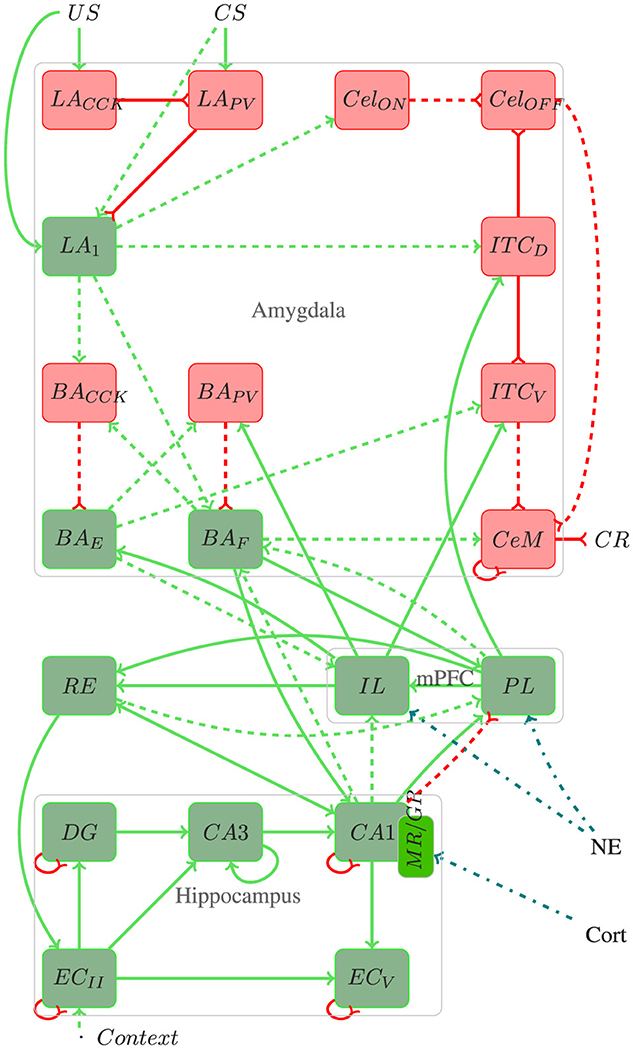
Figure 1. Architecture of the proposed model. Red rectangles and lines represent inhibitory connections, green rectangles and lines represent excitatory connections, blue lines represent stress responses, and dotted lines represent plastic connections. In addition to the elucidated information within the text, pertinent details regarding the number of neurons, connections, and referenced works for each region utilized in the proposed model are provided throughout the text.

The amygdala plays a fundamental role in forming and extinction fear memory, acting as a key processing center for CS−US stimuli and integrating sensory information to influence executive, motor, and memory functions (Akirav and Maroun, 2007; Carrere and Alexandre, 2015). Its sensory input region, the lateral amygdala (LA), receives projections from various cortices, including auditory, visual, gustatory, olfactory, and somatosensory, and is crucial for responding to both conditioned (CS) and unconditioned stimuli (US) (Connor and Gould, 2016).

In the LA, excitatory neurons (LA) coexist with inhibitory neurons containing somatostatin (LASOM), parvalbumin (LAPV), and cholecystokinin (LACCK). The LA neurons, receiving both CS and US inputs, play a pivotal role in encoding fear memories, while LAPV and LACCK modulate these responses through their inhibitory projections (Duvarci and Pare, 2014; Kim et al., 2013; Bennett et al., 2019).

The medial central amygdala (CeM) orchestrates the behavioral, autonomic, and endocrine responses associated with fear, receiving inputs from the LA through various pathways. These include the basal amygdala (BA) pathway, critical for transmitting LA activity to CeM (Pape and Pare, 2010; Asede et al., 2015; Pare and Duvarci, 2012), and the intercalated inhibitory cells, which modulate fear responses during both acquisition and extinction phases (Duvarci and Pare, 2014; Oliva et al., 2018). The lateral nucleus of the amygdala (LA) neurons excite neurons within the basolateral nucleus (BA), which are divided into two distinct sub-populations: one associated with fear acquisition (BAF) and the other with extinction (BAE) (Herry et al., 2008). Also within the basolateral region are inhibitory neurons containing parvalbumin (BAPV) and cholecystokinin (BACCK). Additionally, the lateral subdivision of the central amygdala (CeL) regulates the output of CeM cells, influenced by both US and LA projections (Ciocchi et al., 2010; Mattera et al., 2020; Haubensak et al., 2010; Duvarci and Pare, 2014).

Another critical region of the fear circuit is the medial prefrontal cortex (mPFC). Studies indicate that fear memory extinction requires plasticity in the mPFC and the amygdala (Akirav and Maroun, 2007). The mPFC can modulate the expression of previously learned fear bidirectionally, i.e., it performs coordinated action by integrating several mnemonic inputs and up-down regulation of specific brain circuits (Gilmartin et al., 2014).

The medial prefrontal cortex (mPFC) also contributes significantly to the fear circuit, modulating the expression of learned fear through its connections with the amygdala (Gilmartin et al., 2014; Akirav and Maroun, 2007). The infralimbic (IL) and prelimbic (PL) cortices are integral components of the mPFC, crucial for both the formation and extinction of fear memories. While the PL primarily contributes to fear acquisition, the IL is primarily involved in fear extinction (Marek et al., 2018b). Additionally, they exert top-down regulation on the fear response (Sierra-Mercado et al., 2011; Bennett and Lagopoulos, 2018; Marcus et al., 2020).

Furthermore, the hippocampus and the entorhinal cortex (EC) are integral for contextual fear memory processing, communicating through both the trisynaptic (TSP) and monosynaptic (MSP) pathways. These regions send emotion-related information to the amygdala and mPFC, influencing the encoding and recall of emotional memories (Schapiro et al., 2017; O'Reilly and Norman, 2002; Ketz et al., 2013; Tse et al., 2007; Maren et al., 2013; OReilly et al., 2014).

The nucleus reuniens (RE) connects cortical structures and the hippocampus, significantly influencing contextual fear learning and memories (Bokor et al., 2002; Vertes, 2006). Inactivation of the RE affects acquiring and retrieving these memories, while projections from the medial prefrontal cortex (mPFC) to the RE are essential for inhibiting fear after extinction (Ramanathan et al., 2018).

2.2 Spiking neural networks

The cells of the proposed model use mainly Integrated and Fire (IF) type neurons based on conductance to express the firing dynamics coming from each network layer (Destexhe, 1997). The IF artificial neuron is a model capable of expressing the dynamics of the Spiking Neural Network (SNN), which describes mathematically the properties of biological neurons that generate electrical potential through the cell membrane caused by the change in the conductance of the receptor channel in the presynaptic region (Destexhe, 1997; Gerstner et al., 2014; Raudies and Hasselmo, 2014; Rezaei et al., 2020).

The IF model analyzes neuron action potential propagation through a time-dependent current. When the potential reaches a certain established threshold, it triggers spikes, instantly raising the potential before it returns to its resting value (Abbott, 1999). According to the model, the membrane potential is given by:

CdVidt=-gleak[Vi(t)-E]+Isyn(t)+η    (1)

The input current Isyn drives the membrane, modeled using capacitance C with potential Vi, through the leakage conductance channel gleak, where E represents the synaptic conductance reversal equilibrium potential. The index i represents the ith modeled region. The term η represents small fluctuations in the membrane potential and is a random variable η ϵN(μ, σ), extracted from the Gaussian distribution N with mean value μ and standard deviation σ.

The synaptic current is modeled as the ohmic conductance gsyn multiplied by the driving force, which is the difference between the membrane potential Vi and the reversal equilibrium potential of the synaptic conductance Esyn (Destexhe, 1997).

Isyn(t)=+gsyn(t)[Esyn-Vi(t)]    (2)

Including the excitatory electrical conductivities, gE, and inhibitory electrical conductivities, gI, and considering the membrane potential about the τ refractory period, the membrane potential is given by:

τdVidt=[E-VI(t)]+gEgleak[EE-VI(t)]+gIgleak[EI-VI(t)]+η    (3)

when τ=Cgleak. Furthermore, it has different values for each type of neuron. EE represents the excitatory reversal equilibrium potential, and EI is the inhibitory potential.

When the membrane potential reaches the membrane potential threshold, the neuron fires rise to the peak potential, Vth, and then returns to the resting potential.

Vi→Vresetif(Vi(t)>Vth)    (4)

To update the synaptic weights of IF, we used Spike Time Dependent Plasticity (STDP), an adapted form of Hebbian learning, and frequently implemented in SNN. In the biological context, synaptic plasticity is divided into Long Term Potentiation (LTP) and Long Term Depression (LTD), where LTP represents the changes when a synaptic increase occurs and LTD, a decrease in synaptic gain. STDP suggests that synaptic efficacy increases when presynaptic peaks occur milliseconds before postsynaptic peaks. Likewise, the efficacy decreases when postsynaptic peaks occur before presynaptic peaks (Gupta and Long, 2009).

The model uses a learning mechanism based on physiological data to analyze forwarding and backward temporal order repetition. The weight adaptation is given by:

where Iinf is the hormonal influence.

To represent the influence of corticosteroids in the CA1 region and the consequent increase in the firing of neurons, the percentage of the sparseness of the CA1 region may vary from 10%, standard value, to 50%, saturation value at 40 min after the stressful situation.

2.5 Experimental design

Each experiment is divided into several groups, each performing a specific set of tasks. The timing of behavioral episodes is divided into several phases. In each phase, different initial stimuli trigger unique behaviors or reactions. Furthermore, several cycles of repetition of these behaviors or reactions may occur within each phase. The Table 1 details the correlation between the expressions, the number of cycles and their input stimuli.

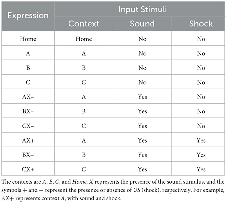
Table 1. Relationship between expressions and input stimuli.

Before initiating any experiment, we establish the computational model's initial configuration through a simulation in the “Home” environment. This process is essential to ensure the neural network's dynamic equilibrium and to prevent any bias in the experimental responses. During this initial phase, we calibrate the synaptic weights, which are adopted as baseline parameters for all subsequent experiments. The simulation in the “Home” environment continues until the output of the central nucleus of the amygdala (CeM) stabilizes below 10% for ten consecutive cycles. This procedure ensures that the network has achieved a state of consistency and robustness, allowing experiments to be conducted with the assurance that the baseline freezing behavior has been adequately controlled and stabilized.

We initialize neurons with a resting potential of −70 × 10−3V, and adjust the membrane potential at each cycle as previously described. After completing the final phase of each experiment, we analyze neuronal activity in the CeM to interpret the network's prediction.

We initiate stress cycles after fifteen cycles of fear acquisition. We selected this threshold of 15 cycles based on baseline factors to activate the norepinephrine and corticosteroid response curves, establishing a reasonable timeframe for stress hormones to begin interacting with the fear acquisition process. Given the various approaches for modeling fear acquisition and transitioning to stress, we chose the 15-cycle mark to introduce stress cycles in a way that reflects a plausible temporal dynamic between fear and stress mechanisms. We adjust stress levels according to Equations 7, 8.

The developed computational model incorporates shock intensity as a configurable variable, enabling the simulation of different levels of unconditioned stimulus (US) intensity by practices observed in behavioral studies. This parameterization allows for replicating variations in behavioral responses found in in vivo experiments.

Additionally, the model maintains a fixed time interval between shocks to ensure consistency in timing during each acquisition phase. The unconditioned stimulus (US) is applied in 2, 000 of the total 8, 000 iterations per phase, ensuring a uniform application of the stimuli. This stringent control of the interval between shocks reflects standard practices in in vivo experiments. Standardizing time between stimuli is essential to minimize variations that may interfere with behavioral responses.

To represent the propagation of the shock effect, the initial current in the sensory layers was set to 1.00nA, ensuring the proper transmission of the stimulus. Additionally, the synaptic current is reduced at a rate of 0.01nA per subsequent layer, simulating the decay of shock intensity as the stimulus progresses through the neural circuit, similar to what occurs in biological systems.

Parameters for configuring the IF neuron include the membrane capacitance (C) set to 5.5pF, and the membrane conductance (Gl) set to 10nS, ensuring that the time constant (τ) is maintained at 0.5ms. The peak potential (Vpico) is set to 0mV. The time interval and step for simulation of the computational model were defined to keep the network frequency close to 8 Hz, representing Theta oscillation. Thus, the time varies close to 125 ms. Each analysis is performed with an interval between 0 and 4, 000 ms and τ = 0.5 ms, resulting in 8, 000 cycles.

Synaptic weights must be modified until the network is appropriately converging to perform all training and testing. They are randomly initialized within the range of values determined by normal distribution, with standard deviation (σ) being 0.3 and mean (μ). Table 2 presents neurons number, connection, mean of the normal distribution, and the design references in each region used on the proposed model.

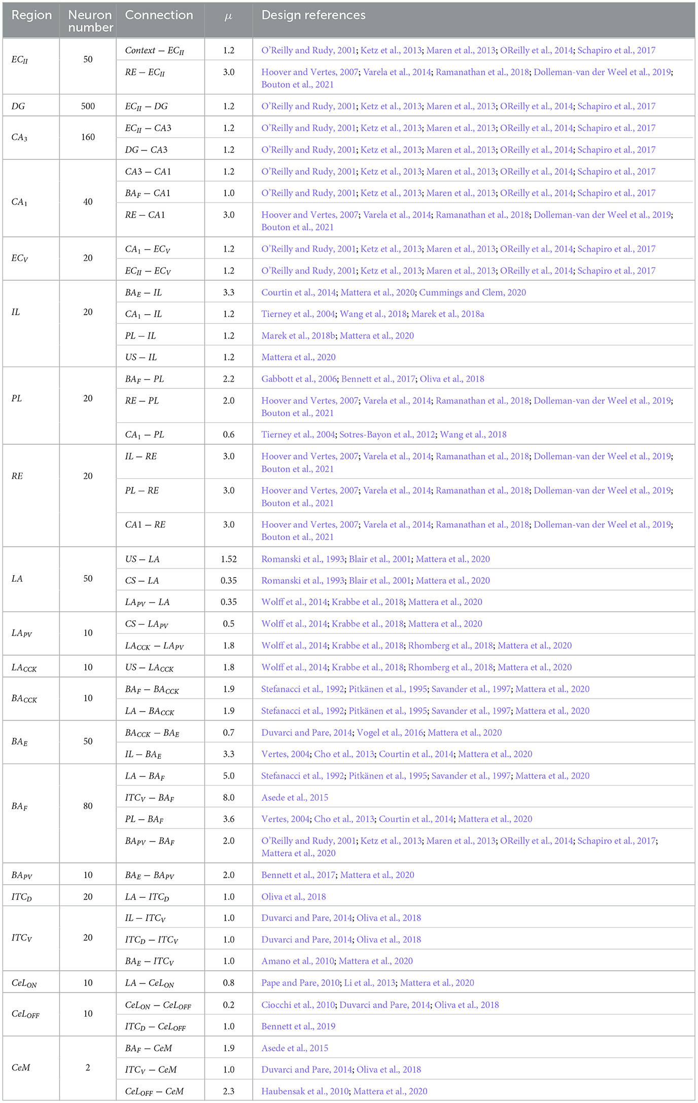
Table 2. Neurons number, connection, mean of the normal distribution, and the design references in each region used on the proposed model.

The STDP synaptic modification rule is used in weights between the layers and the relative time between these layers' presynaptic and postsynaptic peaks. The values needed to parameterize the STDP equation are as follows: the time constant for weight adaptation is 10 τ, the time constant for long-term potentiation (LTP) is 10 τ+, and the time constant for long-term depression (LTD) is 0 τ−. The amplitude for LTP is 1.2 A+, and the amplitude for LTD is -0.4 A−.

The k-WTA function is used to determine hippocampal sparsity in the proposed model. The subregion DG receives 30% of the EC, CA3 receives 5% of the DG, and, finally, CA1 receives between 50% and 100%, in cases of stress elevation. CA3's recurring network is fully wired to help link parts of representation and retrieve patterns from memory. CA1 receives fully connected projection from CA3, and ECV has 50% sparsity.

Table 3 presents all input connections for each group of neurons used in the proposed model. Efforts were made to keep all values low while considering the proportional differences in neuron counts reported in the literature for various brain regions in rats (Boss et al., 1987; Gabbott et al., 1997; O'Reilly and Rudy, 2001; Maier and West, 2003; Chareyron et al., 2011). This approach maintains a realistic ratio of neurons across layers, ensuring both computational efficiency and biological plausibility.

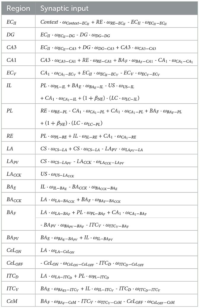
Table 3. Synaptic inputs to each group of neurons.

3 Results

In this section, we expose the results achieved through the application of the proposed methodology, focusing on the evaluation of the neural network through models of contextual fear conditioning (CFC), immediate extinction deficit (IED), and stress-enhanced fear learning (SEFL).

3.1 Experimental consistency and data representation

To ensure the reliability of our experimental outcomes, we rigorously conducted mean and convergence analyses to determine the optimal number of repetitions for each condition, confirming that the observed patterns remained consistent and stable across trials. These analyses also helped establish the minimum number of repetitions required to produce consistent results (Note: Graphs illustrating these analyses are not included in this document). Using the well-known Contextual Fear Conditioning (CFC) paradigm, we observed that the graphical representations of the mean, boxplot, and confidence intervals of the means per number of repetitions began to converge from the fifteenth repetition. At this stage, the confidence intervals stabilized within an upper and lower limit of 5%. Consequently, a minimum of fifteen replicates was deemed sufficient to produce reliable and representative results for the experiments conducted in this study.

We visualize the data using boxplots, which effectively summarize the response distributions within each group. The boxplot format highlights central tendency and variability, allowing straightforward comparison across conditions. In these boxplots, the red “+” symbols indicate outliers-values that fall outside the expected range for each group. This visualization approach underscores the overall trends in the data and provides a solid basis for visually assessing group differences without the immediate need for statistical significance testing.

3.2 Contextual fear conditioning

This experiment consists of three phases: Phase CFC 1, all groups were exposed to five cycles in AX+ for fear acquisition. Phase CFC 2 fifteen cycles of BX− for fear extinction. Phase CFC 3, Group 1, was reintroduced to AX− to assess fear renewal and Group 2 to BX− to assess repetition of extinction. This experiment analyses the process of fear extinction and examines the means of fear renewal after extinction. Table 4 details each step and Figure 3 outlines the maximum freezing level obtained for each phase.

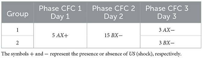
Table 4. Contextual fear conditioning.

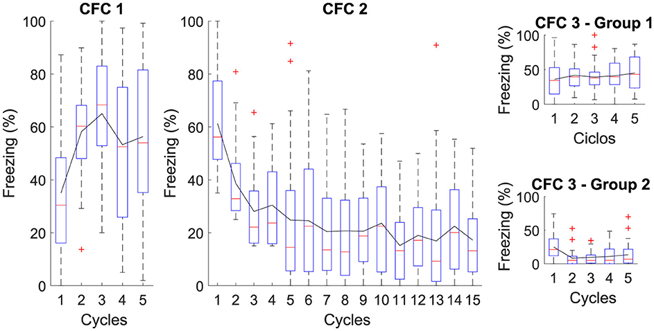
Figure 3. Average level of freezing (%) for Contextual Fear Conditioning: The Figure illustrates the sequential protocol of (CFC 1) fear acquisition, (CFC 2) fear extinction, (CFC 3) renewal, and repetition of fear extinction. In Phase CFC 1, the acquisition occurs for AX+. In Phase CFC 2, Context “B” for extinction is introduced, denoted as BX−. In Phase CFC 3, Group 1 presents renewal and Group 2 with repetition of extinction.

The figure illustrates the average freezing levels (%) across different phases of Contextual Fear Conditioning (CFC). In CFC 1, fear acquisition occurs with high freezing levels, indicating successful learning. In CFC 2, the introduction of a different context for extinction shows a gradual decrease in freezing, demonstrating effective fear extinction. CFC 3 presents two groups: Group 1 presents some fear renewal when the original context is reintroduced, while Group 2 exhibits further reduced freezing levels with repeated extinction. This reduction in freezing is attributed to continued extinction sessions, which result in the CeM receiving more inhibitory than excitatory signals, effectively suppressing the fear response.

The proposed neural architecture and computational modeling enable verifying that the extinction phase is essential to attenuate the association between context and fear, indicating that extinction reduces the existing fear response and makes it difficult to reactivate fear in the same context.

3.3 Fear response at different shock magnitudes during the acquisition phase

The following study investigates the mechanisms underlying the fear response at different shock magnitudes (SM) during the acquisition phase. Specifically, exploring the role of intensity in the conditioned stimulus-unconditioned stimulus (CS-US) pairing provides valuable information about how different threat levels modulate the fear response.

For the simulation, each group, respectively, receives 1, 10, 20, and 30 shocks at the acquisition phase (Phase SM 1). The experiment features fifteen extinction cycles in Phase SM 2. Table 5 and Figure 4 present details of the experiments.

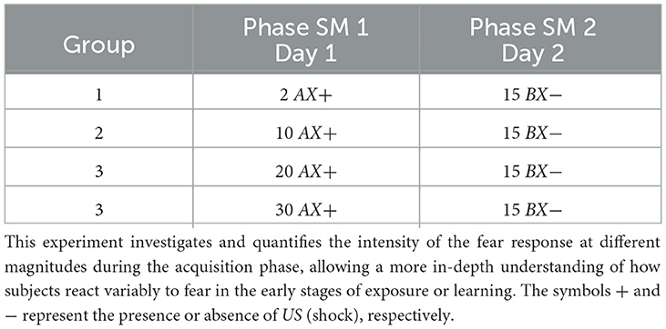
Table 5. Fear response at different shock magnitudes during the acquisition phase.

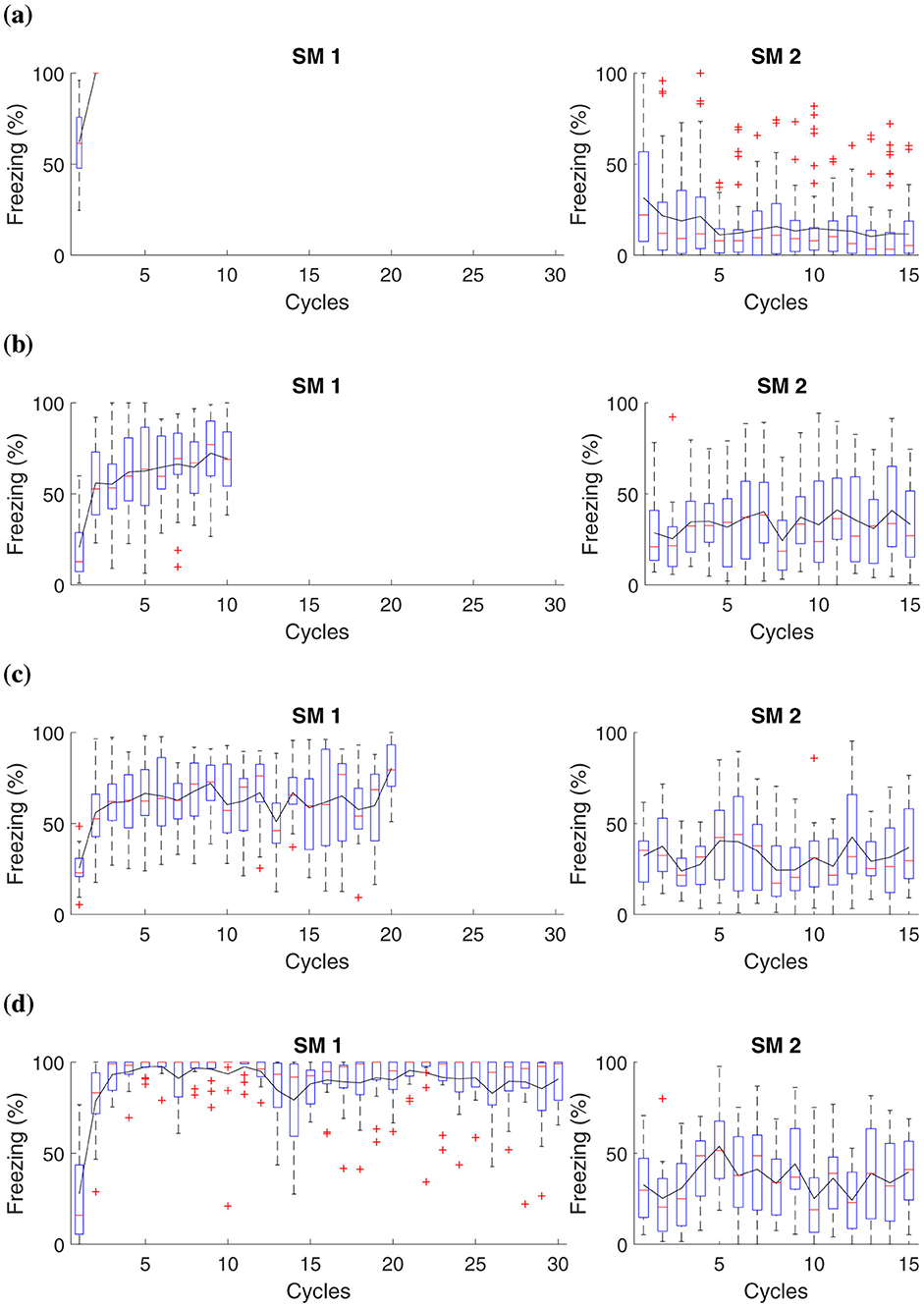
Figure 4. Average freezing level (%) for fear responses at different magnitudes during the acquisition phase. The Figure presents a simulation that captures fear responses at different magnitudes during the acquisition phase. In Phase SM-1, three distinct groups are subjected to different intensities of electric shock in AX+: (A) Group 1 receives a two shocks, (B) Group 2 receives ten shocks, (C) Group 3 receives twenty shocks, and (D) Group 4, thirty shocks. The simulation advances to Phase SM-2 with fifteen cycles in BX−.

This experiment demonstrates that when subjecting animals to shocks of low magnitude, as observed in groups that receive up to two shocks, the intensity may not be sufficient to establish a lasting aversive memory linked to the context or conditioned stimulus. Consequently, these animals demonstrate reduced fear retention.

The results suggest that after administering ten or more shocks, there is already a significant increase in fear retention, as evidenced by higher freezing responses. This marks a tipping point where the intensity and frequency of the unconditioned stimulus (the shocks) begin to consolidate a stronger aversive memory. Consequently, animals exhibit higher freezing rates during extinction, indicating substantial fear retention. Notably, after fifteen cycles, the stress response involving noradrenaline and corticosteroid levels, as described in the Neuromodulation section, becomes fully activated. These hormonal changes reinforce the established fear response, impacting the behaviors observed in Groups 2, 3, and 4 by enhancing alertness and stress regulation over time.

3.4 Stress-enhanced fear learning

Based on the SEFL model, the following experiment investigates the induction of fear learning by stress. During Phase SEFL 1, Group 1, and Group 2 undergo 15 cycles in A, and Group 3 and Group 4 undergo fifteen cycles in A+. In Phase SEFL 2, Group 1, and Group 3 experience a cycle in B, and Group 2 and Group 4 are exposed to a cycle in B+. In Phase SEFL 3, all groups go through a cycle in B. The specific details of the experiment are elucidated in Table 6, while Figure 5 presents the collected data.

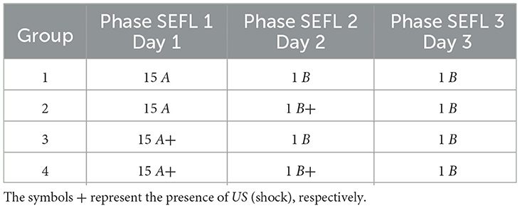
Table 6. Stress-Enduced Fear Learning.

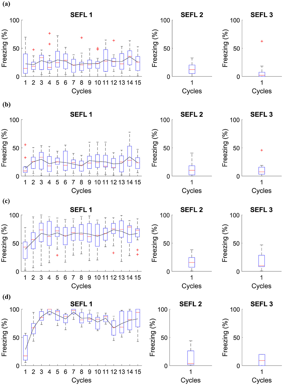
Figure 5. Average level of freezing (%) for fear responses obtained for SEFL. (A) Group 1 goes through Phase SEFL 1, fifteen cycles in A, in Phase SEFL 2, one cycle in B, and in Phase SEFL 3, one cycle in B. (B) Group 2 proceeds with Phase SEFL 1, fifteen cycles in A, Phase SEFL 2, one cycle in B+, and Phase SEFL 3, one cycle in B. (C) Group 3 experiences Phase SEFL 1, fifteen cycles in A+, Phase SEFL 2, one cycle in B, and Phase SEFL 3, one cycle in B. (D) Group 4 undergoes Phase SEFL 1, fifteen cycles at A+, Phase SEFL 2, one cycle at B+, and Phase SEFL 3, one cycle at B.

The experiment reveals different results for each group studied, indicating variations in behavior and response to fear. Group 1 shows no significant changes in its behavior, suggesting a stable response to the experimental conditions. Group 2, on the other hand, exhibits higher freezing levels, a reaction that intensifies after being subjected to a shock in Context B.

Group 3 demonstrates a mild freezing reaction during the testing phase, which is notable considering that the shocks occurred in a context different from that used for testing. This analysis suggests a possible generalization of fear to different contexts.

Group 4 presents a significantly higher level of freezing. This group experienced a previous trauma in Context A and was likewise subjected to a shock in Context B the day before the test. This Group suggests that pre-existing fear, when combined with additional trauma, may result in a more pronounced fear response.

3.5 Shock stress must precede fear conditioning

This experiment analyzed whether previous and prolonged exposure to stress can increase fear responses. In Phase SS 1, all groups were inserted into Context B, with Group 3 and Group 4 receiving a shock. In Phase SS 2, Group 2 and Group 4 receive fifteen shocks in Context A, while Group 1 and Group 3 remain in context A. In Phase SS 3, all groups were submitted to Context B only once, and finally, in Phase SS 4, all groups are inserted into Context A.

The specific details of the experiment are elucidated in Table 7, while Figure 6 presents the collected data.

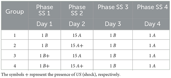
Table 7. Shock stress must precede fear conditioning.

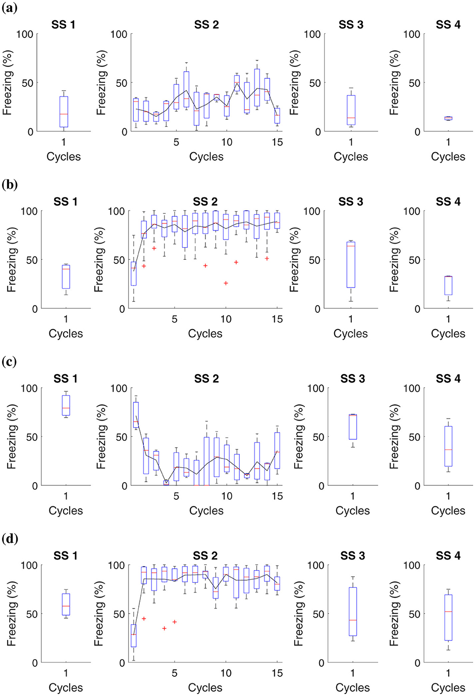
Figure 6. Average level of freezing (%) for fear responses obtained for “Shock stress (SS) must precede fear conditioning.” All groups undergo testing in Context B in Phase SS 3 and Context A in Phase SS 4. (A) Group 1 goes through Phase SS 1, one cycle in Context B, and Phase SS 2, 15 cycles in Context A. (B) Group 2 undergoes Phase SS 1, one cycle in Context B, and 15 cycles with shock in Context A. (C) Group 3 proceeds with Phase SS 1, one shock in Context B, and Phase SS 2, 15 cycles in Context A. (D) Group 4 experiences Phase SS 1, one shock in Context B, and Phase SS 2, 15 shocks in Context A.

In this study, it was possible to observe that prolonged exposure to aversive stimuli, such as shocks, can increase an organism's tendency to develop more intense fear responses in future situations. Previous traumatic experiences amplify the learning process related to fear.

Data analysis revealed that, in animals subjected to a single shock in Context B, the fear reaction levels, measured through immobility behavior, were consistent regardless of having previously been exposed to multiple shocks in Context A. On the other hand, those who did not experience shocks in Context A presented minimal fear reactions in Context B. Experimental subjects who faced 15 shocks in Context A showed a high freezing reaction in this Context. However, this reaction was not altered by what occurred in Context B.

These results suggest that although previous traumatic experiences influence fear sensitivity, the specific fear response is more closely linked to the specific context where the aversive stimulus is experienced than to aversive experiences in different contexts.

3.6 Immediate Extinction Deficit

This experiment is based on the IED model and is used to analyze whether the timing of extinction influences the magnitude of fear in the fear retention phase. The experiment is divided into four groups: (1) immediate extinction, (2) delayed extinction, (3) immediate non-extinction, and (4) delayed non-extinction. Phase IED 1, all groups are exposed five times to Context AX+ to acquire fear. Phase IED 2, Group 1 undergoes five cycles in Context BX− 15 minutes after acquisition, while Group 2 receives the same five cycles in Context BX− but only 24 hours after acquisition. Group 3 goes through five cycles in Context B 15 minutes after acquisition, and Group 4 experiences the same five cycles in Context B, but 24 h after acquisition. After 48 hours of acquisition, all groups are exposed to three cycles in Context CX−. Table 8 presents the experiments related to the model, and Figure 7 presents the collected data.