1 Introduction

Stroke is a prevalent neurological disorder that significantly diminishes the quality of life for affected individuals. Approximately 40% of stroke survivors experience motor impairments (1), with upper limb dysfunction being particularly common. Such impairments lead to challenges in daily activities and work, significantly reducing the quality of life and independence of these individuals. Early rehabilitation is crucial in recovering upper limb function post-stroke (2–4), aiming to maximize functional restoration and enhance overall quality of life. Prior to initiating rehabilitation, a comprehensive assessment of the upper limb is essential to determine the extent of impairment and to monitor rehabilitation progress (5). These assessments provide a scientific foundation for developing rehabilitation plans, evaluating treatment outcomes, and predicting prognosis, making effective stroke rehabilitation assessment a critical component of stroke care.

Currently, the most commonly used clinical methods for evaluating post-stroke upper limb function are traditional scale-based assessments (6), which primarily rely on the subjective evaluations of rehabilitation therapists. For instance, Katia demonstrated that the Fugl-Meyer Assessment can infer motor performance and movement quality in individuals with varying severities of chronic stroke. Li utilized employed the Brunnstrom Assessment to grade stroke patients, while Shamay used scales such as the Wolf Motor Function Test (WMFT) and the Upper-Body Dressing Scale (UBDS) for the psychological measurement of upper limb function in stroke patients (7–9). Although these scale-based assessments offer standardization, repeatability, and multidimensional evaluation, they are also limited by subjectivity, restricted sensitivity, and significant time and resource consumption.

With advancements in medical technology, modern devices for upper limb function assessment now include wearable sensors and upper limb rehabilitation robots (10). Wearable sensors comprise surface electromyographic (sEMG) sensors, inertial measurement units (IMUs), and more.

Muscles control the movement of the body's limbs, and muscle strength is defined as the maximum force muscles that can exert under specific conditions (11). Muscle strength is typically measured indirectly through methods like sEMG and inverse kinematics (12). sEMG is used to detect the electrical currents generated by muscle contractions during neuromuscular activity, which helps analyze muscle function and assess a patient's muscle condition. sEMG sensors measure the voltage changes between two points on the muscle, capturing muscle activity using electrodes (13, 14). These sensors are non-invasive, significantly reducing infection risk, and are widely used in rehabilitation medicine, movement analysis, and muscle fatigue studies (15). For example, Hsu used EMG sensors to study the sequence of muscle contractions in stroke patients transitioning from sitting to standing and Bandini highlighted the importance of the co-contraction index of sEMG in evaluating the clinical motor performance of stroke patients (16, 17).

Inertial Measurement Units (IMUs) are wearable sensors composed of gyroscopes, accelerometers, and magnetometers. They offer advantages such as portability, low cost, and space efficiency, making them widely used in upper limb movement assessment models (18). For example, researchers have employed 9-axis motion sensors to measure 23 components of the Fugl-Meyer Upper Extremity Assessment. Other studies have used wearable inertial sensors and end-effector robots for precise motion tracking in rehabilitation therapy to evaluate feedback support and rehabilitation outcomes. Sensors with IMUs have been used to collect elbow inertia data, employing machine learning algorithms like random forests for spasticity assessment. Additionally, the MPU6050 inertial sensor has been used to measure upper limb movement direction, with results compared to hand movement trajectories recorded by Kinect sensors (19–22).

In clinical research experiments, sEMG sensors and IMU sensors are often used together for rehabilitation assessment. For instance, Mahmoud et al. combined inertial measurement units, Kinect sensors, and sEMG sensors with occupational therapy to evaluate upper limb function in post-stroke patients. Similarly, Pan et al. assessed upper limb motor function in stroke patients using inertial and sEMG sensors (23, 24). Objective assessment of data collected by sensors requires advanced data processing techniques, often involving machine learning (25). Machine learning technologies have continuously advanced the integration of engineering and medicine over the past few years, particularly in areas such as medical diagnostics and neural system regulation and classification (26–30). Modern algorithms like Random Forest and Support Vector Machines often outperform earlier methods (31, 32). When applied to muscle signals, these algorithms have been used for classifying movements and detecting muscle activity anomalies (30, 33, 34). Additionally, hybrid deep networks combining Long Short-Term Memory (LSTM) and Convolutional Neural Networks (CNN) have achieved an average accuracy of 80% in automatically recognizing Brunnstrom stages III, IV, and V (35).

This study utilizes a surface electromyographic signal acquisition system and the MPU6050 six-axis motion sensor to collect sEMG and motion data during upper limb movements. Regression prediction models are then established using Random Forest (RF), Backpropagation Neural Network (BPNN), and Support Vector Machine (SVM) machine learning methods. The model's performance is evaluated using metrics such as the R-Square (R2), Root Mean Squared Error (RMSE), Mean Absolute Error (MAE), and Mean Bias Error (MBE). R2 assesses the model's explanatory power, indicating how well it captures data variability. RMSE and MAE provide measures of error, helping to understand the model's accuracy. MBE reveals systematic bias, identifying areas for improvement. These four evaluation metrics allow for a multidimensional assessment of model performance, enhancing our understanding and guiding future improvements. They also help identify the most optimal algorithm for upper limb muscle strength assessment.

2 Materials and methods

In this study, a left shoulder flexion test was carried out on healthy volunteers to capture sEMG signals from the anterior, middle, and posterior deltoid muscles, along with motion capture data of the left upper limb. The arrangement of the muscle sensors and MPU6050 sensor is detailed in Figure 1. Following data collection, feature extraction was executed, and the participants' muscle strength was documented utilizing a manual muscle testing scale. Subsequently, machine learning regression models were established to comprehensively assess the level of shoulder flexion strength. The models' performance was evaluated using four key metrics: RMSE, R2, MAE, and MBE. The outlined research methodology is depicted in Figure 2.

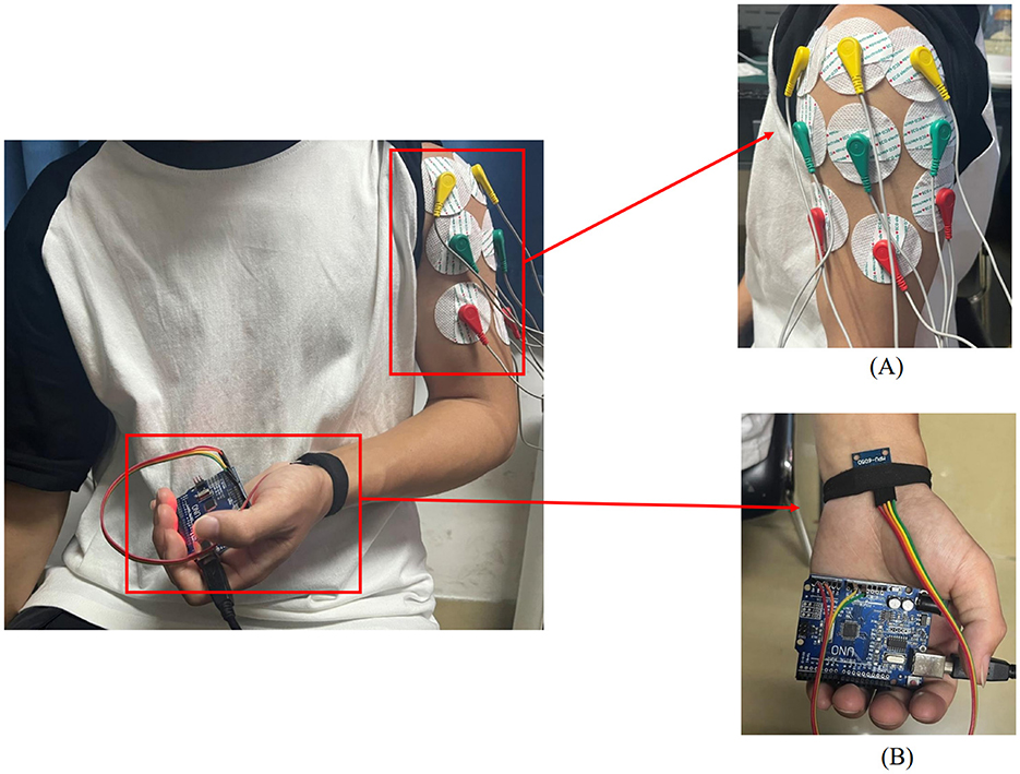
Figure 1. Placement of upper limb testing devices. (A) sEMG sensors are placed on the anterior, middle, and posterior deltoid muscles. (B) MPU6050 sensor is placed at the distal end of the limb.

Figure 2. A method for upper limb muscle strength regression prediction based on sEMG and motion capture. RF, Random forest; BPNN, backpropagation neural network; SVR, support vector regression; RMSE, root mean squared error; R2, R-square; MAE, mean absolute error; MBE, mean bias error.

2.1 sEMG acquisition and analysis

In the process of upper limb movement, capturing muscle changes is essential. Besides feeling muscle contractions through touch, sEMG sensors can be used to collect signals generated during movement.

2.1.1 sEMG signal acquistion system

The electromyography data was collected using a six-channel EMG sensor device, with a sampling frequency ranging from 1,000 Hz to 5,0000 Hz. After testing, it was found that a sampling frequency of 10,000 Hz minimized environmental noise interference. Thus, this study set the final sampling frequency at 10,000 Hz. The setup of the acquisition device is shown in Figure 3.

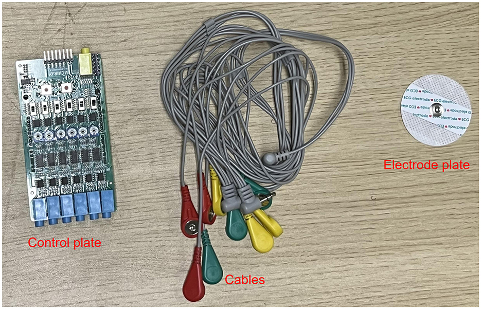
Figure 3. sEMG acquisition device.

In this experiment, shoulder flexion is specified as the motion. The deltoid muscle is one of the main muscles of the shoulder joint, responsible for various movements such as flexion, abduction, and adduction of the shoulder joint. During shoulder flexion, activation of the anterior bundle of the deltoid muscle is most significant. Additionally, the middle and posterior bundles of the deltoid muscle play a supportive role in the stability and support of the shoulder joint. Selecting the anterior, middle, and posterior bundles of the deltoid muscle as the source of sEMG signals allows for a more comprehensive capture of the muscle activity during shoulder flexion, leading to a better understanding of the interaction and coordination among muscles during shoulder joint movements. Therefore, in this experiment, the anterior deltoid, middle deltoid, and posterior deltoid were chosen as the primary data sources for sEMG by analyzing upper limb joint movements. The placement of the EMG electrodes for testing is illustrated in Figure 1A, where the red electrode line indicates the calibration reference point typically positioned at the muscle edge. The yellow and green electrode lines, utilized for sEMG collection, are conventionally placed at the muscle belly. The study focused on shoulder flexion movement of the upper limb and captured the neuromuscular activity of the three deltoid muscle groups during motion.

2.1.2 sEMG preprocessing and feature extraction

sEMG signals are generated from the combination of electrical potentials produced by multiple motor units beneath the skin's surface. Consequently, they are susceptible to noise interference and signal contamination during the data acquisition phase. Utilizing appropriate filtering algorithms is crucial to eliminate noise from various frequency bands (36). In this experiment, a Savitzky-Golay filter was utilized for noise reduction processing. The Savitzky-Golay filter is a type of digital filter that can enhance data accuracy without altering the signal trend or width. Its advantage lies in preserving the characteristic information of the signal while exhibiting good noise resistance. Therefore, in this experiment, the collected raw electromyography signals were denoised using a Savitzky-Golay filter. The key parameters set for the filter during application include window length and polyorder. Here, window length signifies the number of data points considered by the filter in each smoothing computation. In this study, the window length is set to 51, indicating that the filter will consider 51 data points or 51 milliseconds of time for smoothing operations. Polyorder denotes the order of the polynomial used to fit the data in each window. In this experiment, the polyorder is set to 3, signifying that a third-degree polynomial will be utilized for fitting the data in each window. The results post-completion are depicted in Figure 4.

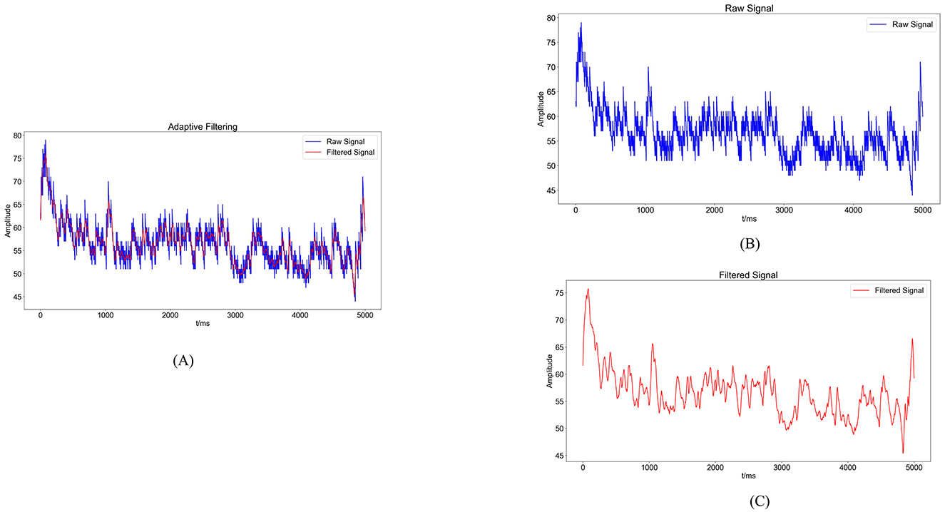
Figure 4. Noise reduction processing results. (A) Comparison graph of original sEMG (blue) and sEMG after noise reduction with the Savitzky-Golay filter (red). (B) Blue waveform represents the variation of the original sEMG. (C) Red waveform represents the sEMG after noise reduction with the Savitzky-Golay filter.

The present study delves into the analysis of sEMG signals by incorporating four time-domain features: Root Mean Square Value (RMS), integral EMG (iEMG), Mean Absolute Value (MAV), and Variance (VAR). Additionally, the feature extracted from the frequency domain includes the median frequency (MF).

The RMS of the sEMG signifies the average of the amplitudes over a specific time interval. It characterizes the average change in sEMG behavior over time, indicating the energy output during muscle activity and aiding in the assessment of muscle involvement in diverse movements.

RMS=1N∑i=1Nx2(i)    (1)

On the other hand, the iEMG refers to the total area enclosed by the rectified and smoothed sEMG curve within a given time unit. It quantifies the cumulative muscle activity during a designated period, illustrating the temporal intensity fluctuations in the sEMG signal over time.

iEMG=1N∑t=1t+T|EMG(t)|dt    (2)

In the equation, EMG(t) represents the collected EMG signal, t denotes the time variable, and T is the period of the EMG signal.

The MAV corresponds to the average of the absolute signal amplitudes within a specific time frame, commonly employed to evaluate muscle contraction intensity and fatigue levels.

MAV=1N∑i=1N|x(i)|    (3)

In the equation: N signifies the number of data points in the collected sEMG, and x(i) denotes the i−th data point in the sequence of the signal.

The VAR is instrumental in revealing the pattern of sEMG dispersion, illustrating the amplitude changes and extent of variations during movement. It is a standard metric for evaluating the motion signal intensity.

VAR=1N∑i=1NXi2    (4)

In the equation, N represents the number of samples, and Xi denotes the amplitude of the sEMG at the i−th sample.

The MF signifies the midpoint frequency of muscle activation during contraction, serving as a reliable indicator of muscle contractile strength and fatigue levels. Typically, the MF decreases with prolonged movement durations.

MF=12∫0∞PSD(f)df    (5)

In the equation, PSD (Power Spectral Density) denotes the power spectrum of the sEMG, and df refers to the sampling frequency.

For sEMG feature extraction, encompassing sample points derived from various movements executed by distinct subjects. Taking the anterior deltoid muscle as an example, the feature values for each sample point are illustrated in Figure 5. Notably, Figure 5 demonstrates significant variances in feature values across different movements, reflecting individual differences in physical conditions and ensuring the data's authenticity.

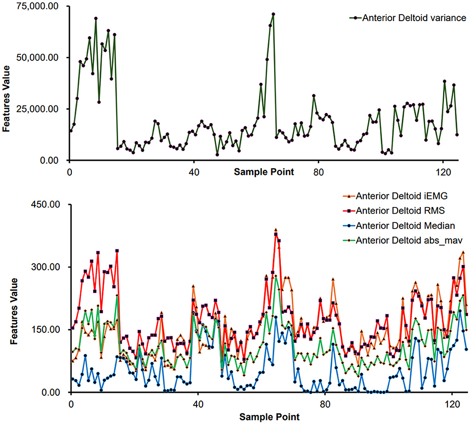
Figure 5. Feature extraction results of different sample points (anterior deltoid muscle).

2.2 Inertial sensor acquisition and analysis

During the upper limb rehabilitation process after a stroke, shoulder joint movements often require compensations as patients may move their scapula or trunk. Preventing compensations during the rehabilitation exercises can enhance treatment effectiveness, as compensations can lead to uncertainty in joint movement angle measurements. This issue of accurately measuring joint movement angles can be addressed by using biofeedback methods such as inertial sensor units.

2.2.1 MPU6050 acquisition device

The MPU6050 is a six-degree-of-freedom inertial sensor that integrates a three-axis gyroscope and a three-axis accelerometer (37). The sensor module utilized in this setup comprises the MPU6050 and Arduino UNO. An orientation calculation algorithm devised with the Arduino IDE software is utilized to assess motion angles and acceleration during movement. During shoulder flexion movements, it is common to maintain the elbow joint in an extended position. The MPU6050 is primarily used to capture angular changes during joint movements and is typically placed at the distal end of the limb, such as the biceps tendon or wrist joint. In this study, the MPU6050 was positioned at the wrist joint as shown in Figure 1B. It was secured using an elastic band to prevent displacement in other directions. Additionally, the connection between the MPU6050 and the UNO board was checked to ensure the stability of signal acquisition.

2.2.2 MPU6050 data acquisition and feature processing

During shoulder joint movement analysis, the MPU6050 sensor is positioned at the distal end of the limb to measure the angular movement of the shoulder joint while maintaining a fixed shoulder position. In this study, the data analyzed consisted primarily of three-axis acceleration, three-axis angular velocity, and three-axis azimuth (yaw, pitch, and roll) obtained from the MPU6050 sensor. The yaw angle refers to rotation around the Z-axis, pitch represents rotation around the Y-axis, and roll signifies rotation around the X-axis. Equipped with three gyroscopes and three accelerometers, the MPU6050 sensor outputs crucial data, including three-axis acceleration (Acc) and three-axis angular velocity (Gyro).

The MPU6050 includes an accelerometer and a gyroscope. The accelerometer calculates roll and pitch angles based on the perceived gravitational acceleration when stationary, with angle calculation dependent on the current position. The gyroscope integrates angular velocity over time intervals to derive incremental angle changes, accumulating these changes onto the previous orientation to obtain a new orientation angle. Therefore, a complementary fusion of the attitude calculated from the accelerometer and gyroscope is performed. The accelerometer estimates object orientation by sensing gravitational acceleration, while the yaw angle, typically used to describe directional changes, represents a rotational angle relative to the horizontal plane. Hence, the gyroscope is essential for capturing yaw angle variations. The overall formula for this integration is as follows:

{roll=roll+(rollacc−rollgyro)*Kpitch=pitch+(pitchacc−pitchgyro)*Kyaw=yawgyro    (6)

In the equation, K is a proportional coefficient that allows the readings from the accelerometer and gyroscope to be fused according to a certain weighted proportion, thereby reducing the impact of noise and drift to achieve a more precise attitude estimation. Typically, the K value ranges from 0 to 1 and can be adjusted based on practical considerations. For this experiment, a value of 0.2 was chosen.

2.3 Prediction model establishment and analysis methods

In this study, we utilized sEMG and motion signals to predict muscle strength recovery using RF, BPNN, and SVM methodologies.

2.3.1 RF regression prediction model

RF is a supervised machine learning algorithm utilized for both classification and regression tasks. This algorithm adopts ensemble learning by combining multiple decision trees to forecast outputs in regression analysis (38). Within the RF algorithm, each decision tree comprises root nodes, intermediate nodes, and leaf nodes, with the path from the root to leaf nodes governed by specific rules. The model's accuracy hinges on the number of decision trees employed, with a bootstrap dataset generated for each tree from the main dataset (39–41). In regression analysis, the RF regression prediction model yields the average of the predicted outputs generated across all decision trees (42).

2.3.2 BPNN regression prediction model

BPNN is a deep neural network trained using the backpropagation algorithm, widely recognized as a mature and extensively employed model in the medical domain (43–45). Comprising an input layer, hidden layers, and an output layer, BPNN derives the inter-layer weights through the iterative process of forward signal propagation and backward error propagation.

2.3.3 SVM regression prediction model

SVM is a supervised learning approach utilized for regression and classification tasks. SVM trains the model using a subset of the training data. In regression contexts, this model is termed Support Vector Regressor (SVR) and excels in handling non-linear, high-dimensional challenges, finding extensive use across clinical, physical, engineering sectors, and other fields (39, 46–48). For regression applications, SVR delineates a “margin band” flanking the linear function to allow deviations until a threshold parameter, ε, is exceeded. Loss computations focus solely on samples outside this band, with the model optimization aimed at minimizing overall loss while maximizing the margin. Introducing slack variables ξ and ξ* quantifies the deviations from the predicted output, with the loss function defined as:

{minw,b,ξi,ξi∗12‖w‖2+C∑i=1m(ξi,ξi∗)s.t.  f(xi)−yi≤ε+ξiyi−f(xi)≤ε+ξiξi≥0,ξi∗≥0,i=1,2,…,m    (7) 2.3.4 Evaluation metrics

In assessing the effectiveness of various machine learning models, it is customary to employ evaluation metrics that elucidate the predictive accuracy of the models. This study utilizes four key evaluation metrics to ascertain the most effective regression method among the three algorithms. The first metric considered is the coefficient of determination (R2), a measure that evaluates the precision of machine learning predictions by providing the squared value of the correlation coefficient R (49). Typically, a satisfactory R2 criterion is set at 0.75, with values exceeding 0.75 indicative of a well-fitted model to the data (46).

R2=1-∑i=1n(Actual valuei-Predicted valuei)2∑i=1n(Actual valuei-Average of outputs)2    (8)

The second evaluation metric is the RMSE, which quantifies the square root of the average squared variance between target and predicted values. A lower RMSE signifies enhanced predictive accuracy of the model.

RMSE=∑i=1n(Actual valuei-Predicted valuei)2n    (9)

The third evaluation metric is the MAE, which works by averaging the absolute differences between the true target values and the predicted values. A smaller MAE indicates higher predictive accuracy of the model.

MAE=1n∑i=1n|Actual valuei-Predicted valuei|    (10)

The fourth evaluation metric is the MBE, which measures the direction of model errors by calculating the average error between predicted values and actual values. A positive MBE indicates that the predicted values are higher than the actual values, while a negative value suggests an underestimation of the actual values. The closer the MBE is to zero, the smaller the bias of the predictive model.

MBE=1n∑i=1nActual valuei-Predicted valuei    (11)

In this study, the R2, RMSE, MAE, and MBE metrics are employed to evaluate and contrast the performance of the machine learning regression models, which are executed utilizing Python.

2.4 Experimental data acquisition 2.4.1 Data collection

This experiment recruited 15 healthy volunteers to participate in the study. The participants were physically healthy individuals without limb injuries, cognitive impairments, or adverse habits. The data collection took place at the Key Laboratory of Medical Information Engineering, School of Medical Informatics, Guangzhou University of Chinese Medicine. Prior to the experiment, all participants were familiarized with the experimental protocol and procedures, and they provided informed consent by signing a consent form. The entire experiment was reviewed and approved by the Ethics Committee for Human Biomedical Experiments at Guangdong Provincial Hospital of Traditional Chinese Medicine.

The sEMG was collected using a six-channel EMG muscle electrode sensor, while the motion data was captured using an MPU6050 inertial sensor. According to the physiological structure of the human body, synchronized sEMG were collected from the anterior deltoid, middle deltoid, and posterior deltoid muscles of the left upper limb of each participant, along with the velocity and angular data during the movement of the left upper limb.

Before testing, the participants cleaned the skin around the muscles with 75% alcohol to reduce low-frequency noise caused by electrode movement due to sweat. During the experiment, the participants remained seated with their elbow joints in a fully extended position. They performed shoulder flexion movements of the left upper limb, and each complete shoulder flexion movement was defined as lifting the left upper limb from the midline of the trunk and returning it to the original position. Each participant performed 10 shoulder flexion movements at different angles. During the movements, the participants also underwent manual muscle testing (MMT) with the assistance of a professional rehabilitation therapist, following the MMT muscle grading standards (as shown in Table 1).

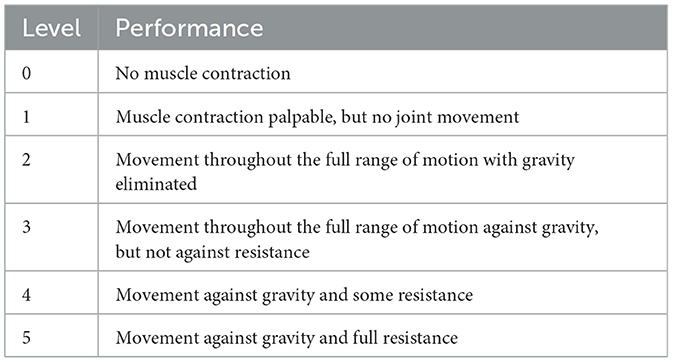
Table 1. MMT muscle grading standards.

2.4.2 Database setup

In this experiment, a total of 15 healthy participants each performed 10 repetitions of shoulde