1 Introduction

Functional magnetic resonance imaging (fMRI) data, particularly resting-state fMRI (rs-fMRI), is inherently complex and high-dimensional. This complexity results in correlated matrices that capture signals from regions of interest (ROIs) in the brain at each time point. Several attempts have been made to analyze fMRI data to understand the roles of ROIs in specific tasks or symptoms (Santana et al., 2022; Wang et al., 2016). Comparing ROIs in fMRI data from different tasks has been one approach to understanding their mechanisms and identifying group differences (Li et al., 2018; Lee and Lee, 2020). However, interpreting which features of ROI connections differentiate between groups has proven challenging for previous studies (Smith et al., 2010; Gates and Molenaar, 2012). There are two main reasons for this difficulty: First, the high-dimensional and correlated nature of fMRI datasets makes it difficult to apply standard statistical models, which typically assume that the data is independent and identically distributed. The complex interactions and dependencies among ROIs in fMRI data make this independence assumption unrealistic, leading to biased or inaccurate interpretations (Smith et al., 2010, 2011). Second, identifying distinctive ROI connectivity that represents group differences is challenging because of the noise introduced by individual effects. Each fMRI dataset corresponds to an independent subject, and the inherent variability and noise in individual effects can obscure the true underlying patterns that distinguish different groups or conditions (Dubois and Adolphs, 2016).

To address these limitations, we propose a novel analytic framework that integrates a deep learning-based classification model with a statistical model, while providing visual interpretation through the functional connectivity networks (FCNs) of ROIs to offer intuitive insights. Since deep learning models are well-known for handling high-dimensional correlated structured data (Du et al., 2022), they are appropriate to apply fMRI data that exhibit complex interactions and dependencies among ROIs. In this study, we utilize a Self-Attention Deep Learning Model (Self-Attn). Self-Attn employs the self-attention mechanism (Vaswani et al., 2017), which is capable of handling correlated structured data and effectively learning adjacency connections (Chen et al., 2018; Zheng et al., 2019; Sun et al., 2020). This enables us to capture intricate connectivity patterns between ROIs in fMRI data. The self-attention mechanism provides an attention distribution for the ROIs, indicating how Self-Attn learns the relationships in the structured input data. Each row in the attention distribution reflects the likelihood of how a specific ROI relates to other ROIs. If the classification accuracy is sufficient, the output of the attention distribution for each subject's ROIs is a reliable source for identifying the ROI connections that distinguish different groups.

However, it is still challenging to identify which ROI connections differentiate groups by manually comparing these distributions. To address this, we analyze the ROIs' attention distribution using the Latent Space Item-Response Model (LSIRM)(Jeon Y. et al., 2021), a statistical network model. We interpret the attention distribution as an item-response matrix (Embretson and Reise, 2013), where ROIs represent items and subjects represent respondents. To the best of our knowledge, there has been no prior research that analyzes the ROIs' attention distribution in the context of statistical network models. Here, the LSIRM estimates relationships between respondents and ROIs by modeling the probabilities of positive responses (connections). This estimation allows our framework to select group-representative ROIs that are consistently shown as meaningful ROIs across all individuals within each group. As a result, our framework effectively tackles the previous challenge of noise caused by individual variations. These distinctive ROI connections are then visualized on the group summary FCN.

The overview of the proposed framework is illustrated in Figure 1, and detailed aspects are presented in Figure 2. Our framework comprises three key steps. In Step 1 (Figures 2A–D), we construct FCNs for each subject's ROIs by connecting them based on their embedded positions using the mapper algorithm (Chazal and Michel, 2017). To manage the time dimension of rs-fMRI data, we first apply dimensionality reduction, and then use the mapper to construct individual FCNs. While this approach reveals the overall connectivity structure, it remains challenging to identify significant ROI connections that distinguish one group from another. In Step 2 (Figures 2E–H), we perform binary classification using Self-Attn (Vaswani et al., 2017) on the subjects' FCNs and generate an attention distribution matrix for each subject. Next, we use the coefficient of variation (CV) and mean values to build a group-level attention distribution matrix. In Step 3 (Figures 2I–J), we apply LSIRM to the group attention distribution matrix to identify group-representative ROIs. These ROIs are then mapped onto a group summary FCN to extend their connections to other ROIs.

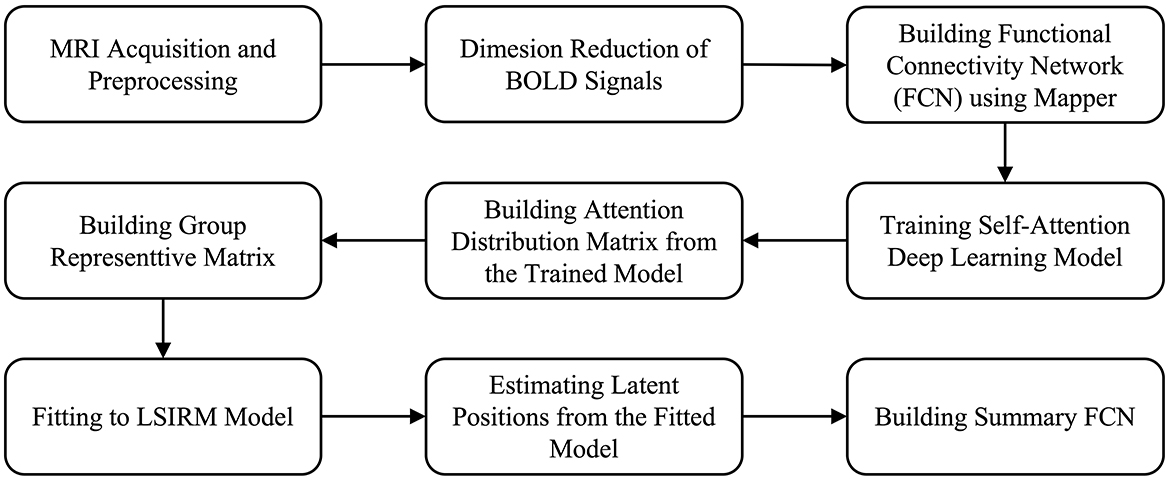
Figure 1. Overview of our fusion analytic framework.

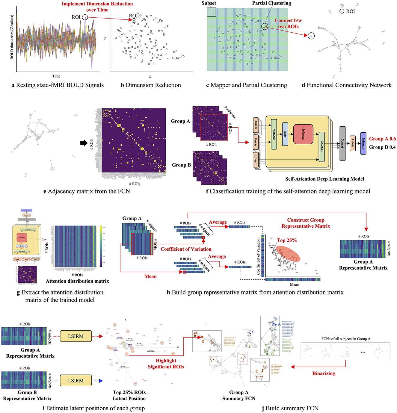
Figure 2. A graphical illustration of the fusion analytic framework with three steps: Step 1 (A–D): constructing the FCN for each group by embedding rs-fMRI BOLD signals into a 2D space using dimensionality reduction; Step 2 (E–H): generating a group representative matrix from the attention distribution matrices; and Step 3 (I, J): identifying meaningful ROIs using LSIRM and marking them on a group summary FCN.

To validate the proposed framework, we applied it to classify rs-fMRI data from different stages of neurodegenerative diseases, which exhibit varying levels of cognitive impairment. We used resting brain scans from the Alzheimer's Disease Neuroimaging Initiative (ADNI) database, which is a multisite longitudinal study widely used for biomarker exploration in Alzheimer's disease diagnosis (Jack Jr et al., 2008; Mueller et al., 2005). We aimed to uncover the distinct features of ROIs between the two groups and compare our results with previous findings from ADNI publications.

2 Materials and methods

Our analysis approach involves three main steps: (1) creating an FCN for each subject in each group, (2) estimating an attention distribution matrix using Self-Attn, and (3) extracting group-representative features of ROIs using LSIRM and visualizing them on the group summary FCN. In this study, we applied our analysis framework to identify the specific ROIs that differentiate four comparisons: Alzheimer's Disease (AD) vs. Mild Cognitive Impairment (MCI), AD vs. Early MCI (EMCI), AD vs. Late MCI (LMCI), and EMCI vs. LMCI. We utilized rs-fMRI data collected from AD, EMCI, MCI, and LMCI groups in the ADNI dataset.

2.1 ADNI study

The ADNI dataset is composed of four consecutive cohorts (ADNI1, ADNI2, ADNI-GO, and ADNI3). Participants were recruited for initial periods in the ADNI1 cohorts (October 2004). Follow-up of participants were recruited to the ADNI3 cohort period. To facilitate the preprocessing of the brain rs-fMRI data, we selected data with the same MR parameters. Among several MR parameters, three MR parameters were applied as criteria (200 time points, TR = 3000 ms, 48 slices). After filtering based on these three conditions, 281 participants remained in the ADNI2, ADNI-GO, and ADNI3 cohorts. The ADNI1 cohort was excluded because it did not contain data that met the aforementioned conditions. As a result, we used axial rs-fMRI data from 57 AD subjects, 93 EMCI subjects, 53 LMCI subjects, and 78 MCI subjects (Table 1, Figure 2A). By focusing on these specific disease comparisons, we aim to uncover the key ROIs that exhibit distinct patterns and contribute significantly to the classification and differentiation of these cognitive impairment conditions. All data are publicly available, at http://adni.loni.usc.edu/.

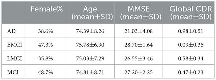
Table 1. Demographic and clinical information (mean ± standard deviation) of the studied ADNI subjects.

2.2 MRI acquisition

The participants included in this study participated in scanning at diverse sites using 3T MRI scanners manufactured by Philips Medical Systems and Siemens Healthineers. The detailed MRI protocols of the ADNI dataset were reported on the webpage (http://adni.loni.usc.edu/methods/mri-tool/mri-acquisition/). In the ADNI2 and ADNI-GO cohorts, MRI scanning was performed at 26 different sites with Philips 3T MRI scanners, using synchronized scanning parameters. In the case of the ADNI3 cohort, Siemens 3T MRI scanners were used to collect fMRI data with synchronized parameters.

2.3 MRI preprocessing

The rs-fMRI datasets, originally formatted in Digital Imaging and Communications in Medicine (DICM), were converted to the Neuroimaging Informatics Technology Initiative (NITI) format, the standard in fMRI research. This conversion preserved all original slices across four dimensions (x, y, z, and time). The preprocessing steps began with slice timing correction to account for the acquisition order of slices, as required by the MRI protocol. Since all rs-fMRI data were acquired using interleaved scanning (an alternating acquisition method), the slice order was applied accordingly, alternating between even- and odd-numbered slices (1 to 48). Following slice timing correction, realignment and head motion correction were performed to address misalignment or movement artifacts.

Next, the corrected rs-fMRI data were spatially normalized to a 3 mm isotropic voxel size using an EPI template, ensuring anatomical consistency across brain MR images. Smoothing was applied using a Gaussian kernel (FWHM = 6 mm, full-width at half-maximum) to optimize spatial resolution and reduce noise. To account for scanner drift and physiological fluctuations, linear trends were removed, and covariates such as white matter (WM) and cerebrospinal fluid (CSF) signals were regressed out, isolating relevant brain activation data. Temporal bandpass filtering (0.01–0.1 Hz) was then applied to minimize low- and high-frequency noise, preserving fluctuations related to intrinsic brain activity.

Finally, the Automatic Anatomical Labeling (AAL) atlas, which segments the brain into 116 regions, was used to define brain regions and extract ROI time-course data. All preprocessing steps were conducted using the Data Processing and Analysis of Brain Imaging toolbox (DPABI, Version 5.3, available at http://rfmri.org/dpabi), and Statistical Parametric Mapping (SPM, Version 12, available at www.fil.ion.ucl.ac.uk/spm/software/spm12/), both implemented in MATLAB R2020b (MathWorks, Natick, MA, USA) (Yan et al., 2016).

2.4 Functional connectivity networks

Dimension reduction methods are well-established techniques for embedding complex and structured data, including Principal Component Analysis (PCA) (Dunteman, 1989), T-distributed Stochastic Neighbor Embedding (t-SNE) (van der Maaten and Hinton, 2008), and Uniform Manifold Approximation and Projection (UMAP) (McInnes et al., 2018). Both t-SNE and UMAP model the manifold using stochastic and topological information. Respectively, t-SNE converts neighborhood distances into conditional probabilities that represent similarity, while UMAP employs a fuzzy simplicial complex with edge weights that reflect the likelihood of connectivity.

2.4.1 Dimension reduction

PCA (Dunteman, 1989) is a technique that uses an orthogonal transformation to reduce high-dimensional data to low-dimensional data (main components) that are not linearly related. The axis with the most significant variance is the first principal component, and the second greatest variance is the second principal component. This decomposition divides the sample into components that best represent the differences. On the other hand, t-SNE (van der Maaten and Hinton, 2008) is a non-linear dimension reduction method that aids in understanding the data with impact information. It is based on t-distribution, which has a heavier tail than normal distribution that helps cover up the far distribution element of high-dimensional data. The t-SNE results depict the embedded points whose distances, trained by calculating the points' similarity in structure, reflect their degree of similarity. UMAP (McInnes et al., 2018) is a nonlinear dimension reduction method that models the manifold using a topological structure. Because it is based on topological space, the embedding points are close in proximity if the two data points have similar topological features. It first reorganizes the data into a fuzzy simplicial complex. This complex produces the connections based on the hyper-parameter that controls the connectivity around the data. Then, it projects the correlated structured data into a low-dimensional space based on their connection, where the connection indicates the proximity.

2.4.2 Mapper

Mapper is one of the techniques derived from topological data analysis, which enables the representation of the topological structure of high-dimensional data as a network. Topological data analysis simplifies the complexity of the topological space by transforming it into a network consisting of nodes and connections that capture the topological characteristics, such as points, lines, and triangles. The Mapper process involves two main steps. First, the high-dimensional topological space is mapped onto a real-valued measure space represented as a graph. This mapping function can be any real-valued function that captures the essential features of the data. For example, dimensionality reduction techniques like PCA, t-SNE, and UMAP use real-valued functions to project high-dimensional data into a lower-dimensional space such as Euclidean space. In the next step, the mapper partitions the graph into subsets of data, and each subset is clustered to define connections. This process identifies the structural relationships within the data. This process is called the Mapper, where each sub-cluster is treated as a node, and nodes are connected when they share similar data attributes.

The Mapper can be considered a form of partial clustering. It applies a standard clustering algorithm to subsets of the original data and examines the interactions between the resulting sub-clusters. When two non-empty subsets U and V are considered, their sub-clusters may have overlapping elements that construct a simplicial complex. The sub-clusters are referred to as vertices (or nodes), while the overlapping elements form edges in the complex. This process yields a simplicial complex consisting of points, lines, and triangles, which provides insights into the topological structure of high-dimensional data.

2.5 Attention distribution matrix

The attention distribution matrix is obtained from Self-Attn, representing a probability distribution that captures the relationships between input elements that play a key role in performing a task. The training phase, as detailed in Algorithm 1, is shown in Figure 2F, where the FCN is trained using Self-Attn. In this phase, the model learns the relationships between ROIs from the input FCN and identifies which network of ROIs characterizes the unique features of a given group. The inference phase corresponds to Figure 2G, where the trained model takes the FCN of a subject as input and extracts values from a specific layer, generating the attention distribution matrix. This layer captures the relationships between ROIs in parallel, in the form of a probability distribution, thus capturing diverse interaction patterns among the ROIs. Finally, these relationships are averaged to produce a single matrix which is called the attention distribution matrix. This matrix explains the relationships between ROIs that contribute to classifying a subject into a specific group.

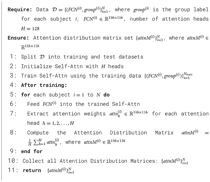
Algorithm 1. Self-Attn for training attention distribution matrix.

In particular, Self-Attn with multi-head self-attention can distinguish between groups but also explains the relationships among ROIs that contribute to group classification. Multi-head self-attention is one of the core mechanisms of the Transformer model. It is highly effective in learning how different elements in input data are related to each other (Vaswani et al., 2017). It is particularly useful for exploring interactions between brain regions (Zhao et al., 2022, 2024). Self-attention evaluates each element's relationships, focusing on the more important elements based on this information. This is particularly useful for capturing the interactions between ROIs and identifying relationships that distinguish groups (Velickovic et al., 2017; Lei et al., 2022; Zhang et al., 2022).

Key components of the multi-head self-attention mechanism, which plays an important role in executing self-attention, are known as Query (Q), Key (K), and Value (V). These components are used to learn the relationships between input elements. Q functions as a ‘query,' capturing how a specific ROI relates to other ROIs. K holds the features of each ROI, encapsulating the information each ROI possesses, and is used together with Q to assess the relevance between ROIs. For instance, if the dot product between Q and K is high, the corresponding ROIs have highly significant interactions. V contains the actual information of each ROI and is propagated using the attention weights derived from Q and K. For example, if a particular ROI receives high attention weights, it extracts crucial information from the V of other ROIs, generating more meaningful outputs.

The input consists of Q, K, and, V, all having a dimensionality of dk. The computation involves calculating the dot products between Q and each K, dividing the result of each by the square root of dk, and then applying a softmax function to obtain weights corresponding to V. If we consider a total of R ROIs, we can represent Q, K, and V as element of ℝR×dk. By applying softmax to the attention scores obtained from the dot product of Q and K, we derive the attention weights, denoted by attn(Q, K). These attention weights represent the relationships between ROIs and indicate the probability distribution of how much each ROI should focus on other ROIs. The final output is obtained by multiplying V with attn(Q, K).

attn(Q,K)=Softmax(QK⊤dk)Attention(Q,K,V)=attn(Q,K)V    (1)

Equation 1 is extended into multi-head self-attention as shown in Equation 2 to capture various aspects of ROIs, particularly in high-dimensional datasets. Here, with H heads, headh where h = 1, ⋯ , H, each headh layer consists of weight matrices WhQ, WhK, and WhV, which applied to the output layer. The multi-head self-attention is formed by concatenating these H sets of headh. The resulting output is passed through a multi-layer perceptron.

MultiHead(Q,K,V)=Concat(head1,...,headH)WO    where  headh=Attention(QWhQ,KWhK,VWhV)    (2)

In the end, we obtain the attention distribution matrix from the trained model via the inference phase (Figure 2G). For each input, the attention distribution matrix attnM(Q, K) is obtained by averaging the attention layers across all H heads, denoted as attnh.

attnM(Q,K)=∑i=1HattnhHwhere  attnh=attn(QWiQ,KWiK)    (3) 2.6 Group representative ROIs features using Latent Space Item-Response Model

LSIRM (Jeon M. et al., 2021) is a model that represents item-response datasets as bipartite networks, estimating interactions between items (ROIs) and respondents (subjects). In our study, we aim to estimate the latent positions of ROIs based on the interactions between subjects and ROIs. Here, the “Interaction” is measured by the degree of value between subjects and ROIs, indicating the association between subjects and ROIs. These patterns are visualized by estimating the latent positions in space, which can be in Euclidean space, allowing for a more intuitive understanding of these associations. The original LSIRM model is designed for a binary item-response data (0 or 1) (Embretson and Reise, 2013). Therefore, we adopt a continuous version of LSIRM to apply it to group representative matrix Xh|g, h. Each cell value yij represents the coefficient of variation of ROI j in the attention distribution of subject i from group h compared to group g. This is continuous for i = 1, ⋯ , Nh, and j = 1, ⋯ , R. Equation 4 shows the continuous version of LSIRM:

ℙ(yij∣Θ)~Normal(θj+βi−||uj−vi||,σ2),    (4)

where Θ represents , β = , U=j=1R, V=i=1Nh} and ||uj−vi|| denotes the Euclidean distance between subject i and ROI j. LSIRM consists of two parts, the attribute part and the interaction part. In the attribute part, there are two parameters: θj ∈ ℝ and βi ∈ ℝ. The parameter βi represents the degree of responses for the subject i, while θj represents the responses for ROI j. In the interaction part, we have the latent configurations uj and vi for each ROI j and subject i, respectively.

If subject i shows a high value in ROI j, the corresponding association is relatively strong, which is represented through their distance uj − vi. Therefore, their latent positions uj and vi become closer because of a smaller distance compared to other associations. Conversely, if subject i shows low values in ROI j, the association is weaker, and the distance between their latent positions uj and vi is comparably larger. Based on the latent positions of ROIs and subjects, we can interpret the overall relationships that are inherent in data. Algorithm 2 outlines the detailed training procedure for LSIRM.

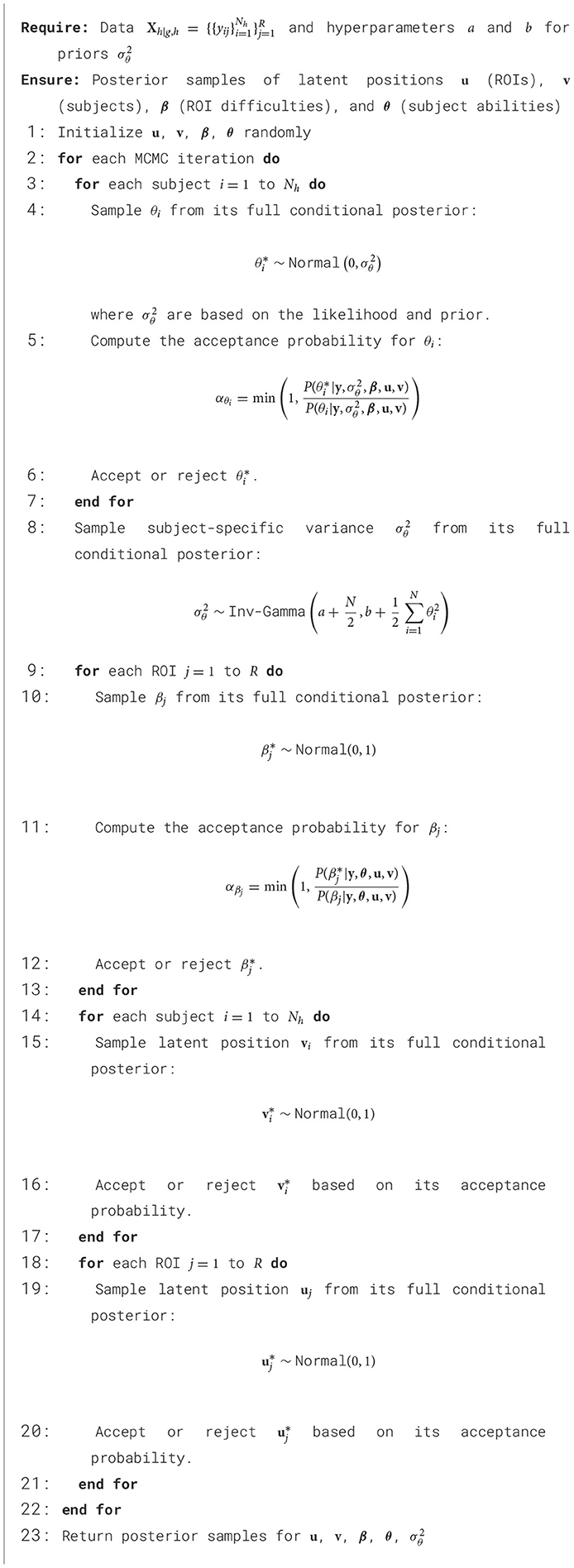
Algorithm 2. LSIRM training process using Markov chain Monte Carlo (MCMC).

Additionally, we can understand the significance of the latent positions of ROIs. When the latent positions of ROIs are located near the center, it indicates that most subjects respond similarly to these ROIs. This is because, when estimating the latent positions of these ROIs, the positions of all subjects are considered simultaneously, resulting in a minimization of the distance between the latent positions. Consequently, the latent positions of commonly reacted ROIs are near the center, allowing most subjects to exhibit similar reactions. This property facilitates the extraction of commonly reacted ROIs for each group h compared to group g, enabling the construction of the group representative matrix Xh|g, h.

2.7 Advantages of Self-Attn and LSIRM in capturing fMRI intricacies

Self-attention (Vaswani et al., 2017) evaluates the relationships between elements in the input sequence, and assigns weights to emphasize important information from these relationships. This mechanism enables the model to consider all interactions between ROIs in a single computation. Furthermore, because it processes all ROIs simultaneously, it is useful for capturing long-range dependencies which helps capture global information. Multi-head self-attention enables learning in parallel interactions between ROIs, allowing the model to capture diverse relationships and patterns in greater depth.

In contrast, eXtreme Gradient Boosting (XGBoost) (Chen and Guestrin, 2016) is an ensemble method based on decision trees that is focused on identifying classification rules between each data element and the target, instead of considering the relationships among elements. In other words, XGBoost classifies based on specific ROI values. However, when data patterns are unclear, such as in rs-fMRI, it is also important to understand the overall network of ROI relationships. XGBoost can have difficulty capturing these complex underlying interactions (Mørup et al., 2010; Mart́ınez-Riaño et al., 2023).

On the other hand, Multi-Layer Perceptron (MLP) (Qiu et al., 2020) primarily analyzes global features instead of local patterns, leading to the loss of information about the interactions between specific ROI features. MLP processes all input data features simultaneously, and as data passes through each layer, it gets transformed using non-linear activation functions. However, this process does not learn the interactions between the inputs, since all inputs are equally processed throughout the network. While MLP can easily capture global characteristics, they have limitations in training complex interactions between ROIs (Lai and Zhang, 2023).

On the other hand, Convolutional Neural Networks (CNN) (Zunair et al., 2020) extract features by sliding small filters over the data. However, it is difficult for CNN to capture global relationships within the data through a single convolution operation. To address this, multiple layers are required, which necessitates more data and increases the training time needed to learn global relationships. While CNN is effective at learning local interactions between adjacent ROIs, they have limitations in capturing the global interactions between ROIs (Wang et al., 2018).

For these reasons, Self-Attn is particularly well-suited for learning interactions between ROIs, as it can simultaneously capture local information and global patterns. This capability makes Self-Attn effective at capturing the complex signals within rs-fMRI data. As shown in Table 2, this results in superior performance compared to other models.

Our approach uses LSIRM to visualize the interactions among ROIs, reflected in the group representative matrix derived from the attention distribution matrix. LSIRM captures these interactions by estimating the latent positions of ROIs, providing an intuitive interpretation of their relationships. Importantly, the group representative matrix is not an adjacency matrix, but a subject-by-ROI matrix, where the goal is to identify group-level features rather than individual-specific ones. Since LSIRM considers all subject-ROI interactions, it identifies common ROI features that show consistent reactions across all subjects. Therefore, by employing LSIRM, our approach can achieve a better understanding of group effects and provide a more intuitive way to interpret ROI interactions.

3 Results

In this study, we applied our analysis framework to identify the specific ROIs that differentiate between four disease comparisons: AD vs. MCI, AD vs. EMCI, AD vs. LMCI, and EMCI vs. LMCI. We utilized rs-fMRI data collected from AD, EMCI, MCI, and LMCI from the ADNI dataset.

3.1 Step 1: functional connectivity networks of each group

First, we constructed an FCN among brain regions based on their rs-fMRI Blood-Oxygen-Level-Dependent (BOLD) signals. We used AAL-116 templates to extract 116 rs-fMRI BOLD signals, representing different brain regions. Supplementary Table S1 in supporting information contains detailed information about the AAL-116 templates. Due to the high-dimensional and correlation structure of fMRI data, we implemented dimension reduction such as PCA, t-SNE, and UMAP over time to embed the high-dimensional correlated structure dataset into low two-dimensional space (Figure 2B). We empirically searched for the optimal combination of UMAP hyperparameters to enhance prediction accuracy. Based on this, we chose the number of neighbors to be 15 and set the minimum distance to 0.1, consistent with hyperparameters used in previous studies for visualizing high-dimensional data, such as genomics (Becht et al., 2019) and single-cell data (Diaz-Papkovich et al., 2021).

To mitigate the subjectivity in determining relevance among ROIs, we employed Mapper (Chazal and Michel, 2017), a partial clustering method, to identify significant connections between ROIs (represented as Figure 2C). ROIs assigned to the same cluster were considered connected. Subsequently, we generated FCNs for each set of embedded ROIs from different dimension reduction methods (represented as Figure 2D). These FCNs captured relationships and connectivity patterns within the high-dimensional correlated fMRI data, representing the data as a connectivity network.

Figure 3 and Supplementary Figures S1–S3 show each subject's rs-fMRI BOLD signals and two types of FCNs: correlation- and dimension-reduction-based FCNs obtained from dimension reduction methods corresponding to AD, MCI, EMCI, and LMCI. Through correlation- and dimension-reduction-based approaches, those different perspectives enabled a comprehensive understanding of their structural characteristics. Note that these FCNs are input for Self-Attn to classify between two diseases. One can apply other dimensionality reduction methods to obtain the embedded ROIs; however, one can select the optimal method based on the prediction accuracy provided by the Self-Attn, where the input is FCNs.

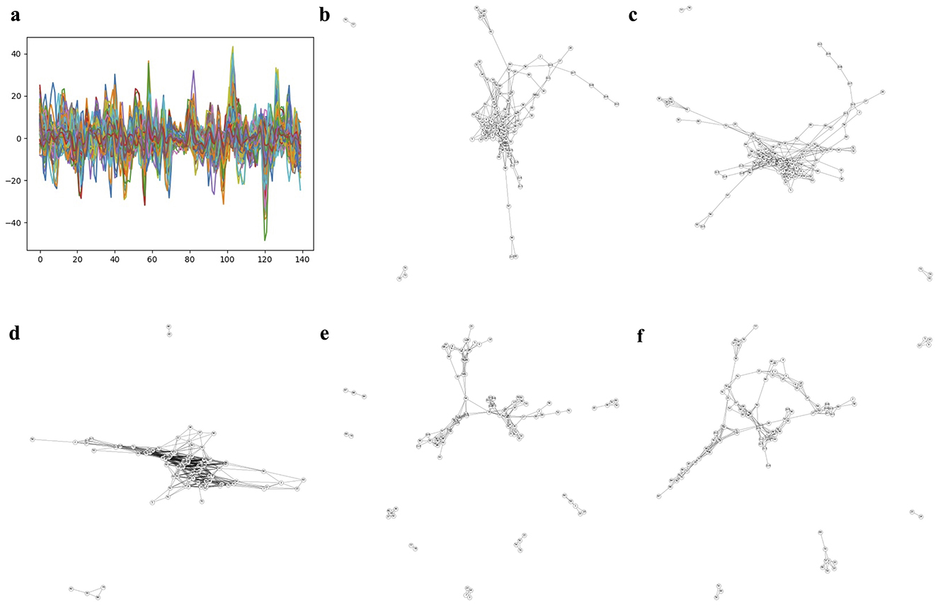
Figure 3. Correlation- and dimension reduction-based FCNs for an AD subject. (A) shows ROIs and rs-fMRI BOLD signals for an AD subject. FCNs were generated using correlation-based methods: Pearson's r and Fisher's z (shown in B, C). To better understand the interrelationships between brain regions, dimension reduction techniques were applied to estimate latent positions of ROIs: PCA in D (linear space), t-SNE in E (stochastic space), and UMAP in F (topological space).

3.2 Step 2: attention distribution matrix from self-attention deep learning model

We focus on identifying which ROIs are important features for distinguishing groups in terms of ROIs' interactions with others. In the previous step, we applied dimension reduction techniques such as PCA, t-SNE, and UMAP to the original time-series of the ROIs to construct FCNs. Additionally, we compared these findings with two correlation matrices calculated from the original time-series data of the ROIs: (1) Pearson's r and (2) Fisher's z, both of which capture the associations among ROIs. With this data, we employed Self-Attn, using FCNs or correlation matrices as input, with the target being a binary indicator of group membership.

In the Transformer architecture, dk is typically defined by dividing the total input dimension (dmodel) by the number of attention heads (h) (Vaswani et al., 2017). However, the roles of the various attention heads vary, and not all heads contribute equally to model performance. Therefore, focusing on the most important heads can maintain model performance while reducing the risk of overfitting (Voita et al., 2019; Michel et al., 2019). To optimize classification accuracy while avoiding overfitting and underfitting, we conducted a parameter search for h = . By modifying h, we implicitly explored the corresponding dk as well, specifically investigating dk = where setting dk to a small value is practically effective specifically in self-attention (Tay et al., 2022). We validated the model through a 10-fold cross-validation, and showed that the configuration with h = 128 and its corresponding dk = 2 achieved consistently robust classification performance. We provide details for parameter search in Supplementary Figure S4. We applied the model to 116 ROIs using the following settings: the batch size of 8, a dropout rate of 0.9, Adam optimizer (Kingma and Ba, 2014), the learning rate of 0.01, and cross-entropy loss.

Table 2 shows the performance of Self-Attn. We compared the classification performance against recent studies (Liu et al., 2020; Wee et al., 2019) and baseline models [XGBoost (Chen and Guestrin, 2016), MLP (Qiu et al., 2020), and CNN (Zunair et al., 2020)]. Our method outperforms all other approaches across the disease group comparisons. Notably, the stochastic and topological-based FCN, which captures hidden connectivity among ROIs, achieved the highest accuracy.

Using Self-Attn, we obtained the attention distribution (Figure 2F) by each ith subject from group g. These attention distributions, denoted as A(q,r)(i)∈ℝ116×116, where i = 1, ⋯ , Ng. Here, Ng indicates the number of subjects from each disease group g = , where NAD = 57, NMCI = 78, NEMCI = 93, and NLMCI = 53. These attention distributions A(q,r)(i) reveal the features that the model focused on when classifying subjects in each disease group against the other comparison groups.

We considered this attention distribution A(q,r)(i) as the matrix Yg|g,h(i), for g ≠ h and g, h = 1, ⋯ , G, where each row and column corresponds to ROIs, and the values indicate the significance of each ROI's contribution to the classify the subject i in group g against group h (Vig, 2019) (Figure 2G). Although the resting-state data shows low signal levels, the classification accuracy of 90% demonstrates that the attention matrices effectively distinguish between the two disease group comparisons.

Figures 4, 5 and Supplementary Figures S5, S6 represent attention matrices for four randomly selected subjects from the AD and MCI groups, respectively. These matrices are the outcomes of Self-Attn employed for AD and MCI classification, utilizing FCNs derived from topological dimension reduction techniques as inputs. ROIs with Higher attention values suggest their significance in classifying subjects. For instance, in Figure 4A, Putamen_R shows a higher attention value, which is a consistent result in Putamen's volume in the AD group (de Jong et al., 2008). Furthermore, Angular and Paracentral areas have high values indicating that Self-Attn focuses on these regions to assign this subject to the AD category over MCI. Similarly, in Figure 4B, Supplementary Figure S5A, Caudate_R, Caudate_L, ParaHippocampal_L, Cerebellum, Cingulum_Ant_L, and Cingulum_Ant_R have high values which also show significant ROIs marker in AD group (Kesslak et al., 1991; Bobinski et al., 1999; He et al., 2007; Catheline et al., 2010).

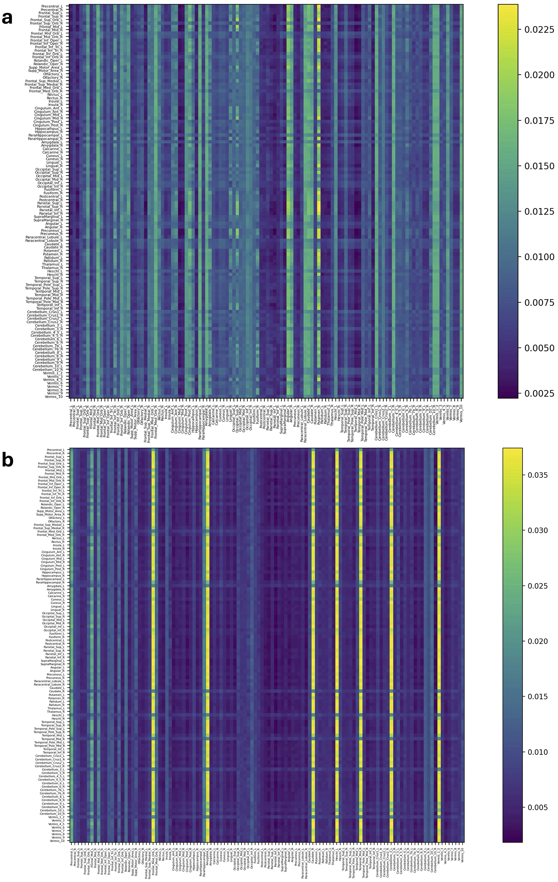
Figure 4. Attention distribution matrix of two subjects within the AD group (A, B), generated by Self-Attn designed for AD and MCI classification, utilizing topological-based FCNs as input.