1 Introduction

Atrial fibrillation stands as the most prevalent sustained cardiac arrhythmia, carrying an elevated risk of heart failure, vascular embolism, and sudden death. Timely diagnosis and intervention are pivotal in enhancing patients’ cardiac function and reducing mortality rates. Late gadolinium enhancement magnetic resonance imaging (LGE-MRI) provides a comprehensive view of cardiac structural morphology and function. The assessment of the LA in LGE-MRI images holds crucial clinical significance, including planning and guidance of atrial fibrillation ablation, postoperative follow-up studies, fibrosis quantification, and biophysical modeling (Aschauer et al., 2016; Khurram et al., 2016). However, the small left atrial cavity, enclosed by the thin atrial wall and featuring complex anatomical structures such as irregular protrusions and discrete multiple targets (Maceira et al., 2010; Wang et al., 2019; Xiong et al., 2021), poses challenges. Moreover, adjacent anatomical structures, such as the left ventricle, often exhibit similar image intensities, making accurate identification more difficult. While manual segmentation could reconstruct and explore the atrial structure, it typically necessitates specialized domain knowledge and incurs high labor costs (Oakes et al., 2009). Additionally, manual atrium segmentation is time-consuming, error-prone, and highly subjective (Petitjean and Dacher, 2011; Caudron et al., 2012). Therefore, the development of an automatic segmentation method with high precision for the LA holds substantial scientific significance and practical value as an auxiliary tool for medical diagnosis, treatment planning, prognosis, and related applications. Traditional segmentation methods, based on regional growing (Karim et al., 2008) and atlas guiding (Zuluaga et al., 2013), encounter limitations due to poor image quality and individualized variations in anatomical structures. In contrast, deep learning methods, renowned for their exceptional segmentation accuracy, possess the ability to automatically learn image features and have extensive applications in image segmentation (Litjens et al., 2017). The U-Net network (Ronneberger et al., 2015), a variant of Fully Convolutional Network (FCN) (Long et al., 2015), has been widely adopted for medical image segmentation since 2015. Building upon the success of 2D U-Net, 3D deep learning networks, such as 3D U-Net (Çiçek et al., 2016) and V-Net (Milletari et al., 2016), have been developed to directly process 3D volumetric data and generate 3D volumetric segmentation results. In the domain of atrial segmentation, deep learning has been the focal point of comprehensive research (Drozdzal et al., 2016). modified the network structure by introducing short-skip connections to FCN, achieving notable segmentation results without post-processing operations (Yang et al., 2020). proposed a joint segmentation method, combining spatial consistency from multiple views with a recursive attention module for LA and scar segmentation in 3D LGE-MRI images (Wong et al., 2022). Proposed a novel GCW-UNet architecture, incorporating Gaussian blur and channel weight neural network for automatically segmenting the left atrial region in MRI images of patients with left atrial enlargement (Uslu and Bharath, 2023). Presented a quality control method based on the multi-view network TMS-Net. The approach significantly improves noise robustness and run-time quality estimation for cardiac MRI segmentation through an innovative design featuring a single encoder and three decoders (Raj Singh et al., 2023). Introduced ARW-Net, a deep learning-based segmentation approach with attention-guided residual links and upgraded deep supervision, showcasing its potential as an outstanding solution for automated and generalized cardiac segmentation. Numerous studies have integrated deep learning methods with traditional approaches or incorporated prior knowledge into deep learning networks to obtain more anatomically reasonable segmentation results. For instance, (El Jurdi et al., 2020), integrated position and shape information into the convolutional layers of the model, guiding the model to identify the target structure’s location and fine-tuning network parameters under a fully supervised learning framework.

Despite the significant progress achieved by deep learning methods in atrial image segmentation, challenges persist, particularly in data imbalance and effectively segmenting blurred edges. In cardiac MRI images, the LA or its margins serve as small structures, contributing to class imbalance issues within the data due to their limited size. Approaches to addressing class imbalance encompass techniques such as image cropping and cascaded networks. For instance (Xiong et al., 2020), employed two continuous Convolutional Neural Networks (CNNs) for atrium segmentation. The first CNN identifies the region of interest, while the second CNN is utilized for target structure segmentation. Based on the 3D U-Net (Vesal et al., 2020), developed a two-stage architecture encompassing coarse and fine segmentation, achieving end-to-end learning. In contrast to cropping or cascaded network methods (Kausar et al., 2021), addressed class imbalance by leveraging prior knowledge and posterior handling operations, utilizing a dense V-Net for segmentation, and fine-tuning parameters. In addition (Kausar et al., 2023), proposed a 3D shallow residual segmentation network based on the 3D multi-scale residual learning structure, introducing a composite loss function and parameter adjustment to tackle class imbalance in medical image datasets without pre-processing and post-processing. Despite successful LA segmentation, these methods exhibit limitations, such as information loss in cropping or cascaded network approaches, redundancy in two-stage architectures, challenges in ensuring model robustness, susceptibility to subjective judgments and empirical influences in designing composite loss functions and adjusting parameters. Additionally, efforts have been made to tackle the challenge posed by the indistinct edges of target structures (Huang et al., 2022). applied the distance map associated with the target structure’s edge as a weight map and utilized a two-stage network to improve LA segmentation performance (Uslu et al., 2022). designed a multi-task segmentation network that integrated edge information of the image into decoding modules of multiple scales. Nevertheless, these methodologies did not fully leverage the available edge information, limiting their effectiveness in addressing the challenges posed by blurred boundaries.

Therefore, to improve the performance in atrial boundaries, this research introduces an EIEM capable of optimizing segmentation by learning and reinforcing boundary information of the target structure, accompanied by a specifically designed Spatially Weighted Cross-Entropy (SWCE) loss function that constrains the module. The contributions of this work can be summarized as follows:

• A novel EIEM was developed to enhance the edge information for image segmentation by integrating edge features with region features. Channel attention modules and multi-scale structural feature fusion are incorporated for edge information learning, enhancing the model’s attention to crucial edge feature channels and the model’s capacity to capture diverse-scale structures and details.

• In this study, we innovatively designed a SWCE loss function tailored to the EIEM to address the class imbalance in the dataset. This loss function incorporates dynamic weighting for positive and negative samples, allowing for adaptive adjustments. Combined with image cropping, the customized loss function effectively mitigates class imbalance in a flexible and data-driven manner.

• The SWCE loss function adapts to the significance of each area through its distance-sensitive weighting scheme, aiming to effectively leverage edge details and alleviate challenges posed by fuzzy edges in segmentation. Supplemented by the Cross-Entropy loss linked to the target region segmentation network, the SWCE loss encourages the model to prioritize edge regions and enhances flexibility.

• The proposed framework is validated on the 2018 Atrial Segmentation Challenge dataset, demonstrating superior performance compared to state-of-the-art methods, especially regarding average symmetric surface distance. The integration of edge constraints improves segmentation outcomes, particularly for irregular protrusions and discrete multiple targets.

The paper is organized as follows: Section 2 provides a detailed introduction to our model; Section 3 outlines the experimental methodology; Section 4 discusses the experimental results; and Section 5 concludes the paper.

2 Materials and methods2.1 Datasets

The datasets utilized in the proposed method are sourced from two distinct collections:

2018 Atrial Segmentation Challenge dataset (Xiong et al., 2021): The dataset used comprises 100 3D LGE-MRI images. While the dataset included additional test cases, only the 100 training cases were utilized in our study as they were the primary dataset provided for training and validation during the challenge. These cases were considered sufficient to meet the experimental requirements. Each set of images consists of an original image and a corresponding ground truth (GT) label. The original images cover the full LA, and the GT labels include the intact left atrial cavities and part of the pulmonary veins annotated by domain experts. The spatial resolution of these images is 0.625 × 0.625 × 0.625 mm³. Each 3D volume comprises 88 slices along the Z-axis, and the image dimensions are either 640 × 640 or 576 × 576 pixels. The grayscale values in the original images range from 0 to 255. For the GT labels, the grayscale value is 0 or 255, and a grayscale value of 0 denotes the background class, while a value of 255 designates the area constituting the GT label.

MSD heart dataset (Simpson et al., 2019; Antonelli et al., 2022): This dataset consists of 20 annotated MRI scans, each containing approximately 100 2D image slices, capturing the entire heart at a single cardiac phase. The images were acquired under free-breathing conditions, with ECG gating, using a 1.5T Achieva scanner. The voxel resolution for these scans is 1.25 × 1.25 × 2.7 mm³. Labeling of the left atrium, including the left atrial appendage, mitral plane, and portal vein end points, was performed using an automated tool, followed by the expert’s manual corrections to ensure high accuracy. A key characteristic of this dataset is the small sample size combined with significant variability across the images, which was used to evaluate the generalization performance of the model trained on the 2018 Atrial Segmentation Challenge dataset.

2.2 Pre-processing

Since the MRI images show that the proportion of the LA is small, there is a class imbalance between the foreground class, composed of the LA, and the background class, consisting of other anatomical structures. The learning process tends to focus on the large background class, resulting in poor segmentation of the LA. Moreover, some images consist of inconsistent dimensions. Therefore, based on the positional information of the LA, in this study, the images are first center-cropped to 300 × 300 pixels (from the 2018 Atrial Segmentation Challenge dataset) or 130 × 130 pixels (from the MSD heart dataset) to increase the proportion of the region of interest in the image and then resized to fit the same size of 256 × 256, aligning with the network’s input requirements. The difference in cropping sizes arises from variations in the proportions of the LA within the images, with the cropping sizes being roughly selected to ensure that the background is reduced while retaining the entire LA in all cases. Moreover, data augmentation is applied to the training set through a randomized combination of transformations, including rotation, translation, and scaling, in line with the conditions that may be encountered during medical image acquisition. This operation introduces diversity into the data, augmenting the presence of noisy data, while also mitigating the impact of variations in cropping sizes. The inclusion of a variety of data and the introduction of additional noisy data can enhance the model’s robustness and generalization capabilities.

For both datasets, the data is split into 60% for training, 20% for validation, and 20% for testing. Each data set used for network training consists of images, corresponding GT labels, and generated edge images. Both GT labels and generated edge images are binary, with foreground regions set to 1 and background regions set to 0. The erosion operation is utilized to extract the edges from the GT labels.

2.3 Edge information enhancement segmentation network

In this study, the 2D U-Net network serves as the backbone architecture for learning the region features of the target anatomy. The U-Net network comprises nine blocks, each with two continuous 3 × 3 convolution layers. Following pre-processing, the input images are fed into the network. After two successive 3 × 3 convolutions in the encoder block, down-sampling is performed through the max-pooling process since the max-pooling operation can retain more texture information compared to the average-pooling. The decoder block also contains two successive 3 × 3 convolution layers, followed by up-sampling achieved through deconvolution. The batch normalization and dropout layers are used in the network as regularization techniques to mitigate overfitting. The Relu activation function is applied in feature extraction layers, while the sigmoid activation function is employed in classification layers.

The EIEM concentrates on learning edge features of the target anatomy from the backbone network, while also integrating the learned edge details back into the backbone network. Initiating from input images, the network’s learning process diverges into two distinct directions: learning region features through the backbone network and extracting edge features through the EIEM, which complement each other. The network produces two main outputs: the predicted label images and the predicted edge images for the LA. The final segmentation results are obtained by post-processing the predicted label images by extracting the maximum connected component.

2.3.1 Edge Information Enhancement Module, EIEM

Edge information plays a critical role in accurately delineating the boundaries of the target and improving overall segmentation accuracy. To learn and enhance the edge information of the target structure, an EIEM is introduced, as illustrated in Figure 1. The EIEM first learns edge features from the backbone network at multiple scales and integrates these multi-scale features. These learned edge features are then fed back into the backbone network for additional reference. The EIEM takes the input image and region feature maps as inputs, and the outputs are edge feature maps of the target structure. The input image, as well as outputs of the first four blocks in the backbone network, serve as inputs for the branches of EIEM, constituting a total of five side branches. The first side branch (EIB1) directly takes the original image as input and perceives global image information, which can capture finer-grained features. These low-level features typically contain more details and texture information, which helps to improve the model’s sensitivity to input images and enhance edge feature extraction. This branch integrates with the backbone network by receiving input directly from the image and providing comprehensive edge details that enhance the global context for subsequent processing stages. The inputs of other side branches (EIB2-5) receive region features of the target anatomy at different scales from the backbone network. Two sequential 3 × 3 convolution operations are subsequently employed to extract the edge features from the multi-scale region features. The resultant feature maps are then up-sampled to match the input image size, aligning with region features from the output of the backbone network. Within this submodule, regularization constraints, including batch normalization and dropout layers, are applied.

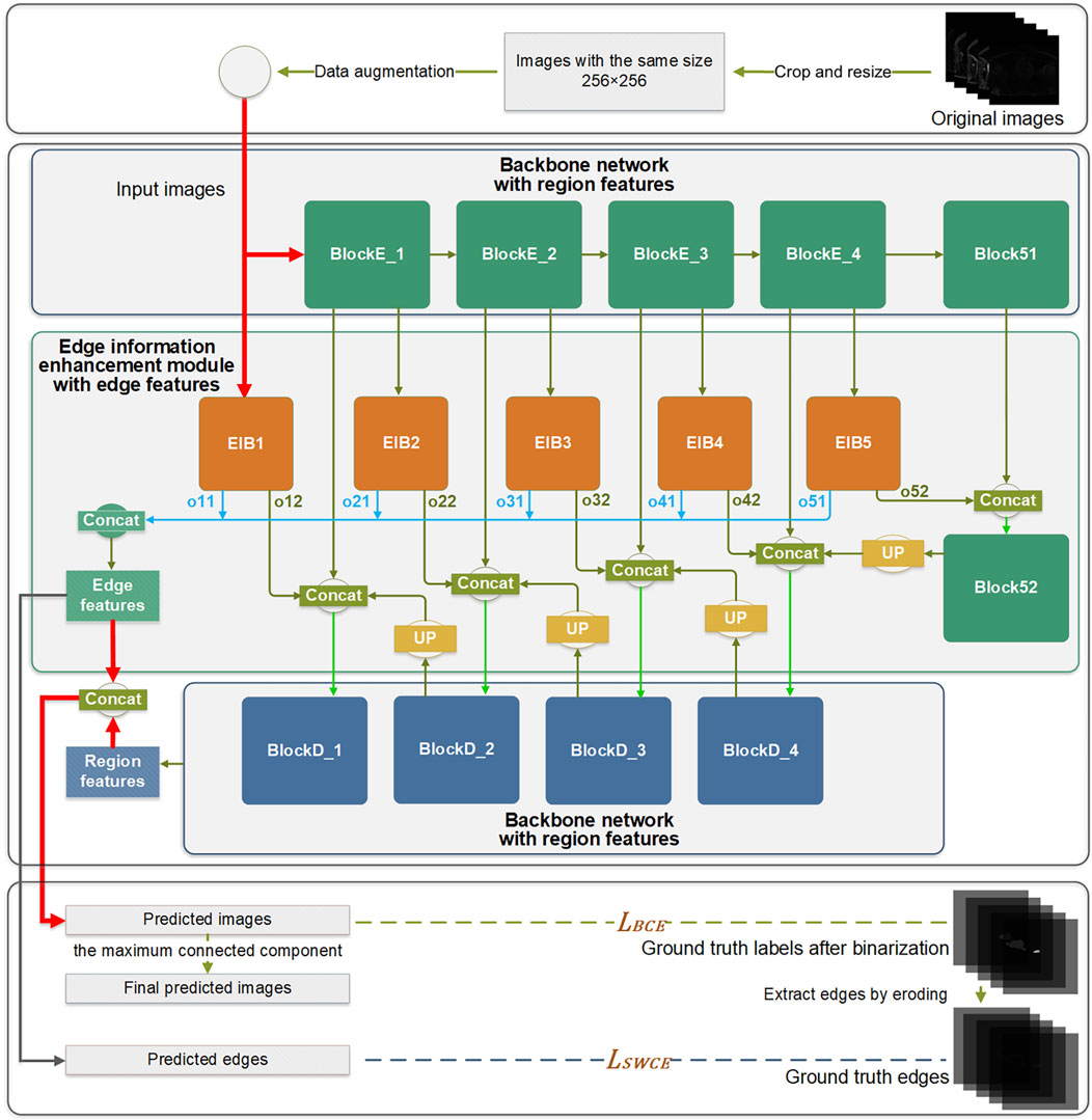
Figure 1. The overall architecture of the proposed method.

Within the edge information block (EIB), channel attention (Hu et al., 2018) is applied to enhance the network’s learning capacity for edge details by focusing on channels containing crucial edge-related information of the target structure. The dynamic adjustment of channel weights by channel attention enables a selective suppression of channels deemed less relevant to edge segmentation, thereby reducing the computational burden associated with processing redundant information. This mechanism is integrated into the backbone network by optimizing feature representations before combining them with the region features from the backbone. Due to its superior performance and low computational cost, channel attention significantly enhances the network’s ability to capture critical edge information while reducing computational redundancy.

Each EIB yields two outputs: the edge features at the original image size (oi1) and the edge features before undergoing up-sampling (oi2), as depicted in Figure 2. The oi1 outputs are fused and processed to obtain the final predicted edge images, constrained by the SWCE loss to optimize the EIEM’s performance in edge segmentation. Concurrently, the fused edge features are combined with the region features learned by the backbone network to enhance the network’s overall segmentation performance on the target, constrained by Binary Cross-Entropy (BCE) loss. Furthermore, the oi2 outputs are integrated with the region features from the decoder parts of the backbone network, providing additional edge information for learning atrial region features and ensuring the preservation of sensitivity to the edge throughout the decoding process. These comprehensive integration and fusion processes with the backbone network, guided by SWCE and BCE losses, ensure the model’s effectiveness in capturing and delineating edges and reinforce the overall accuracy of the model’s segmentation outputs.

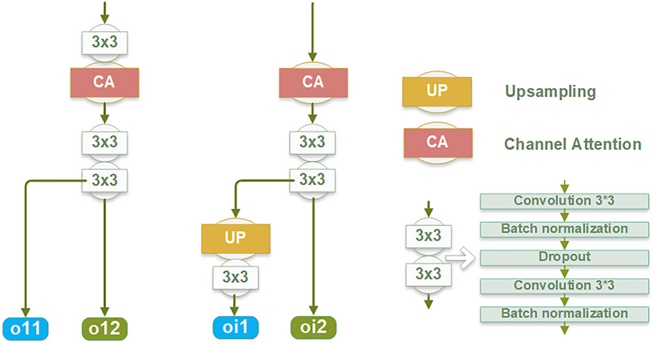
Figure 2. The structure of the edge information block (EIB).

2.3.2 Loss functions

The network incorporates two loss functions: the Binary Cross-Entropy Loss (LBCE) associated with the target region segmentation network and the Spatially Weighted Cross-Entropy Loss (LSWCE) pertaining to the EIEM. The comprehensive loss (L) of the network is the weighted summation of these two losses, expressed by the formula (Equation 1):

where wa and wb are set the values 0.5 each, representing the weighted coefficients for the two losses.

BCE loss is selected for its ability to achieve a better balance between sensitivity and specificity in segmentation results, exhibiting greater stability and a propensity to converge more readily toward the global minimum throughout the optimization process. The BCE loss function of the network is as follows (Equation 2):

LBCE=−y∗⁡logy^−1−y∗⁡log1−y^(2)

where y denotes the value of GT labels and y^ denotes the value of predicted images.

The left atrial edges occupy only a tiny region in a thoracic LGE-MRI image, with the background class covering a significant proportion of the data. Therefore, the SWCE loss function of the network is designed based on the weighted binary cross-entropy loss function to ensure a balanced impact of foreground and background classes on network learning. Further, the SWCE loss function introduces additional parameters to dynamically modulate the importance of pixels based on their spatial characteristics and mitigate class imbalance through dynamic weights assigned to positive and negative samples during computation. The formulation of the loss function is defined as follows (Equation 3):

LSWCEy,y^=−1N∑i=1Nc⋅yi⋅logy^i+1−yi⋅log1−y^i⋅wi(3)

where N represents the total number of pixels in the image, yi denotes the GT label for pixel i, y^i represents the predicted probability for pixel i, and wi signifies the spatial weight of the pixel i. The spatial weight wi is computed based on the pixel’s proximity to the edge. wi and yi are given by the following expressions ( Equations 4, 5):

wi= a,if yi=1 b+1d_to_ei,if yi=0 and ∃j,yj=1 b,if ∀i, yi=0(4)yi= 1,if d_to_ei≤d−1 0,otherwise(5)

where d_to_ei is the Euclidean distance from pixel i to the nearest edge pixel. In Equation 5, the method for thickening the edge inward involves an erosion operation, with the default that pixel i is inside the edge. The parameters a, b, c, and d in Equations 3–5 play crucial roles in the SWCE loss function, governing edge weighting, weight decay rate, class-wise weighting, and edge range, with each serving specific purposes in improving segmentation performance. These parameters are designed to address challenges related to boundary precision and handling class imbalance.

Firstly, parameter a serves as the edge weighting and is introduced to enhance the model’s sensitivity to edges. Assigning higher weights to edge pixels encourages the model to focus more on capturing fine boundary details. This is particularly important in cases where the target structure is small, complex, or irregularly shaped, as these challenging characteristics make it more difficult for the model to capture and differentiate fine boundary details. In such scenarios, the model must be even more sensitive to subtle edge variations, making the role of parameter a crucial for improving segmentation performance.

Secondly, parameter b governs the weight decay rate based on the pixel’s distance from the edge. This helps manage the class imbalance between the large background and the small foreground regions by reducing the influence of background pixels farther from the edge. Combining the reciprocal of the d_to_ei with parameter b achieves a weight decay mechanism, assigning higher weights to pixels closer to the edges and lower weights to those farther away during loss computation, thereby emphasizing pixels near the boundary. Since pixels near the boundary often contain critical transitional information between different regions, focusing on them allows the model to capture fine boundary details more accurately. When b is set to a smaller value, the sensitivity of loss weights to distance increases, prompting the model to focus more on pixels near the edges and emphasize the learning of edge details. Conversely, with a larger value of b, the sensitivity of loss weights to distance decreases, allowing the model to process the entire image smoothly. This design enables flexible adjustments to the model’s focus on different regions of the image, balancing the importance of pixels in the image and enhancing its ability to learn edge information.

Thirdly, parameter c functions as the class-wise weighting to address the class imbalance, helping to balance the contributions of positive and negative samples during training. By tuning c appropriately, the SWCE loss function adjusts the relative importance of positive and negative samples, ensuring the model effectively learns from both classes. This adjustment leads to a more balanced performance across classes.

Lastly, parameter d denotes the edge range. By expanding d - 1 layers inward, the annotated edge region is broadened, providing a more extensive context of the edge features for supervision, which aids in learning more robust edge representations. A larger d value extends the edge region, allowing the model to capture more contextual information around the boundary, which is beneficial for learning the structural characteristics of the edge. However, an excessively large d value may introduce unnecessary complexity. Therefore, the value of d should strike a balance between capturing sufficient context and avoiding overcomplication. Additionally, d will further affect the calculation of w in Equation 4 due to its impact on the y-value of pixels.

Together, these parameters enable the SWCE loss function to focus on edge regions, manage class imbalance, and provide flexibility in how different areas of the image are weighted during training. Their careful selection and tuning, as demonstrated in our ablation studies, contribute to optimizing the model’s performance in image segmentation tasks, enhancing its fine-grained perception of target structures and segmentation accuracy.

2.3.3 Metrics

The proposed method uses the Dice coefficient (DC), Jaccard coefficient (JC), and average symmetric surface distance (ASSD) as metrics to assess the validity of the results.

The DC quantifies the overlap between GT labels and predicted images, with values between 0 and 1. A higher DC signifies a larger overlapping area, indicating a better outcome. The formula for the DC is as follows (Equation 6):

where A represents the GT labels, B denotes the predicted images, A∩B signifies the intersection of A and B. A and B denote the sum of the voxel values of the images. The JC is a metric used to assess the similarities and differences between GT labels and predicted images. A higher JC value indicates a greater similarity between the two. The formula for the JC is as follows (Equation 7):

where A∩B represents the intersection of A and B, and A∪B denotes the union of A and B. The ASSD is chosen as the metric for assessing the segmentation results in terms of distance. The unit of ASSD is in millimeters, quantifying the average distance between two surfaces in the images. A smaller ASSD value indicates a closer alignment between GT labels and predicted images, reflecting a better segmentation result. The formula for the ASSD is as follows (Equation 8):

ASSDA,B=ASDA,B+ASDB,A2(8)

in which Equation 9 is given by the following expression:

ASDA,B=Σa∈Aminb∈Bda,bA(9)

where ASDA,B denotes the Average Surface Distance between volumes A and B, and da,b represents the Euclidean distance between pixels a and b. A signifies the number of surface voxels in volume A.

To further evaluate the performance of the proposed method, we compute the mean and standard deviation (std) of the metrics (DC, JC, ASSD) across test cases. The mean reflects the average performance of the segmentation, providing a central tendency across cases. Meanwhile, the standard deviation quantifies the consistency or variability of the segmentation results. A smaller standard deviation suggests more stable performance, while a larger one indicates greater variability across test cases. Together, the mean and standard deviation offer insights into not only the overall effectiveness of the segmentation method but also its stability across various conditions.

3 Experiments and results

Due to the challenges posed by edge blurring and the similarity in grayscale values of adjacent tissues in medical images, the segmentation of boundary details of the target structure presents a challenging task. In response to this challenge, the study introduces an edge information enhancement design and conducts multiple sets of ablation experiments to demonstrate the effectiveness of the proposed method.

Our model was implemented using the Keras framework (version 2.11.0) and operates on a workstation equipped with an NVIDIA GeForce RTX 3090 GPU. The operating system is Ubuntu 22.04, and the Python environment uses version 3.8. Additionally, CUDA 11.2 and cuDNN 8.1 are employed for GPU acceleration. We employed the Adamax optimizer with polynomial decay to adjust the learning rate during training, starting with an initial value of 0.001. The model was trained for 200 epochs, with the DC on the validation set monitored throughout the training process. The DC on the validation set continuously improved and stabilized around the 200th epoch. As the final model, we selected the parameters that achieved the highest DC on the validation set, ensuring optimal segmentation performance during testing. For further details on the code and environment setup, please refer to the following GitHub repository: https://github.com/PencilSC/EIEM, where we provide the code and necessary configurations to facilitate reproducibility.

3.1 Performance evaluation of the proposed framework

To assess the performance of the proposed model, this study compares it with several state-of-the-art segmentation models on the 2018 Atrial Segmentation Challenge dataset, including nnU-Net (Isensee et al., 2021). The quantitative comparison results, based on three evaluation metrics, are presented in Table 1. In contrast to the other methodologies enumerated in Table 1, the presented approach demonstrates superior performance regarding the ASSD. Meanwhile, the Dice and Jaccard coefficients of this study achieve results comparable to other state-of-the-art methods.

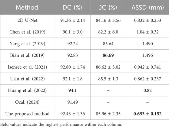
Table 1. Performance comparison between the proposed method and other methods for LA segmentation based on DC, JC, and ASSD with ± std following the values.

Although the algorithm proposed in this study ranks fourth in DC and third in JC, the experimental results show that our algorithm yields slightly lower performance than the methods proposed by Huang et al. (2022), Bian et al. (2019) in terms of Dice and Jaccard coefficients, with only a small difference in values. Meanwhile, our proposed algorithm achieved a significantly improved ASSD result of 0.693 compared to Huang et al.'s 0.82 (the best result of assessed algorithms) and Bian et al.'s 1.496. This enhancement indicates that our algorithm can more accurately capture the manually segmented LA. Compared to other methods, our proposed algorithm enhances boundary information, resulting in more accurate segmentation outcomes, which is crucial for clinical diagnosis and treatment planning. Accurate boundary segmentation can assist clinicians in identifying pathological areas better and provide support for surgical navigation and treatment efficacy evaluation. The lack of notable differences in Dice and Jaccard coefficients may be attributed to factors such as dataset characteristics, data pre-processing, algorithm architecture, and implementation details.

3.2 Ablation and analysis3.2.1 Number of branches

The encoder progressively reduces the size of the feature maps through multiple pooling operations. In the shallow layers of the U-Net, where the resolution of feature maps is higher, fine details such as edge information are preserved. To investigate the impact of varying the number of side branches on the experimental outcomes, ablation experiments were conducted, specifically targeting the number of lateral branches to assess the method’s performance. Starting with the shallow layers, the encoder part utilizes one to five branches for learning edge information. These results illustrate the impact of varying lateral branch quantities on method performance, assessed via DC, JC, and ASSD, as presented in Table 2. Increasing the number of branches from one to five shows improved segmentation performance, especially in capturing fine edge details, as evidenced by higher DC and JC values and lower ASSD values. The incorporation of channel attention modules and multi-scale structural feature fusion enhances the model’s ability to focus on crucial edge feature channels and capture diverse-scale structures and details. Therefore, despite the progressive reduction in resolution as the number of branches increases, fine details such as edge information are preserved. Deeper layers capture high-level semantic information, while shallow layers retain fine-grained details. By incorporating edge information at multiple scales, the proposed method effectively utilizes both high-level semantic context and low-level fine details, leading to more accurate segmentation results.

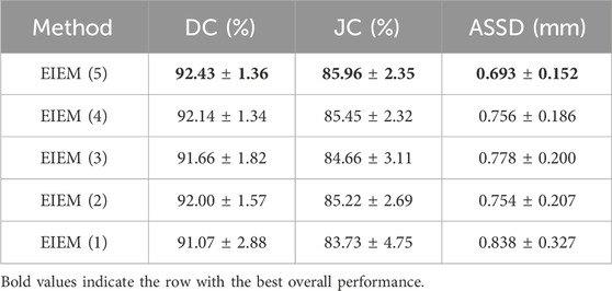
Table 2. Ablation experiments assessing the impact of varying lateral branch quantities on the proposed method’s performance, evaluated through DC, JC, and ASSD with ± std.

The boxplots in Figure 3 visually represent the distribution of the Dice coefficients and average symmetric surface distances corresponding to the numerical data in Table 2. These boxplots complement Table 2 by providing a clear and comparative view of the data’s variability, making it easier to identify patterns and trends across different branch configurations, which may not be immediately apparent from the tabular data alone. In boxplots, data variability is typically illustrated by indicators such as the interquartile range (IQR) or the overall width of the distribution. A wider IQR indicates higher variability, while a narrower IQR suggests more consistent performance. Other aspects include the central tendency, which is represented by the median line in the boxplots, a robust measure that is unaffected by outliers. For instance, while integrating EIEM improves segmentation accuracy overall, particularly in capturing subtle edge details, the impact of varying branch quantities on the mean DC appears less pronounced, which could be attributed to factors like object morphology complexity, image noise, or inherent model limitations. The boxplots show how DC values are distributed for each configuration, with wider spreads indicating higher variability in segmentation performance. This variability is also evident in the higher standard deviation reported in Table 2, which reflects similar distribution patterns. However, the boxplots provide a more comprehensive view by including the IQR, which, along with the overall distribution, offers additional insights into data distribution and is more robust to outliers compared to the standard deviation. On the contrary, the number of branches significantly impacts the ASSD results, exhibiting a noticeable decrease in the mean ASSD with an increasing number of branches, reflecting better boundary accuracy. The boxplots reinforce this observation by showing a more concentrated ASSD distribution as branch numbers increase, reflecting improved consistency in boundary delineation. Although the performance improvements are not strictly linear, the overall trend shows enhancement as network complexity increases. EIEM(5) achieves the best balance between network complexity and data characteristics, delivering optimal performance across the evaluated metrics.

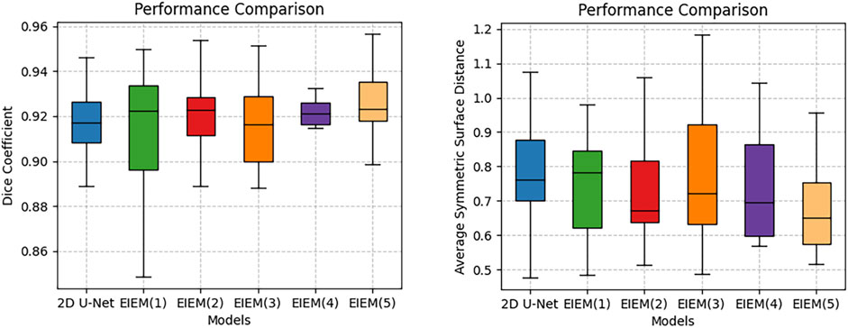
Figure 3. Boxplots of DC and ASSD for models with different side branch numbers.

Figure 4 illustrates the visualization outcomes of models employing varying numbers of branches. For clarity, only the image edges are shown. Each row corresponds to an image along with its segmentation results from different models. GT labels are highlighted in red, while predicted images are depicted in green. EIEM branches significantly contribute to improving segmentation accuracy and enhancing edge detection. As the number of branches increases, there is a more precise delineation of object boundaries, particularly in detecting the edge of prominent terminations. This is evident from the closer alignment observed between predicted edges (green) and GT edges (red).

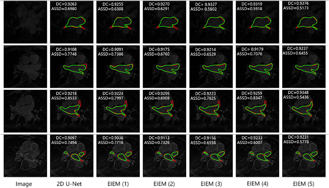
Figure 4. Segmentation results of models with different side branch numbers (In the top left corner are the metrics for the corresponding 3D data). Predicted edges: green; GT edges: red.

3.2.2 The SWCE loss function

Ablation experiments were conducted to analyze the impact of different parameter settings (a, b, c, d) for the SWCE loss function on the network’s performance, as elucidated in Table 3.

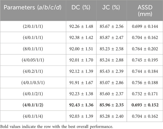
Table 3. Ablation experiments investigating the optimal parameter settings for the SWCE loss function, evaluated through DC, JC, and ASSD with ± std following the values.

The parameter a controls the weight assigned to pixels located on the edges. To identify the optimal value for a, we tested a range from 2 to 8 (2, 4, 8). The results indicated that lower values (e.g., 2) did not sufficiently emphasize edge details. Conversely, higher values (e.g., 8) improved edge detection but showed diminishing returns and potential overemphasis on edge pixels. The intermediate value of 4 was found to strike the best balance. This suggests that moderate edge weighting improves the model’s ability to capture boundary details without excessive focus on the edges, thereby optimizing segmentation performance. Parameter b adjusts the rate at which the weight of pixels decreases with increasing distance from the edge. We evaluated values ranging from 0.05 to 0.2 (0.05, 0.1, 0.2). Smaller values (e.g., 0.05) led to a steep weight decay, focusing excessively on edge pixels and diminishing the representation of background pixels. Larger values resulted in a more gradual decay, which balanced the influence of edge and non-edge pixels but sometimes (e.g., a value of 0.2) reduced the emphasis on crucial edge features. The value of 0.1 was optimal, providing an effective balance that improved segmentation performance by adequately considering pixels both near and far from the edges. The class-wise weighting parameter c balances the contributions of positive and negative samples during training. Parameters a and d increase the weight of positive samples, while the weight decay mechanism reduces the weight of negative samples. Together with c, these factors shape how the model learns from each class. We explored values from 0.5 to 2 (0.5, 1, 2) for c. Lower values (e.g., 0.5) did not adequately weight positive samples, affecting the model’s ability to learn from the minority class. Higher values (e.g., 2) increased the weight of positive samples but could lead to reduced sensitivity to negative samples. The value of 1 provided the optimal balance, ensuring effective learning from both positive and negative samples and mitigating class imbalance. The parameter d defines the range of pixels considered around the edge, extending the annotated edge region inward. We tested values ranging from 1 to 4 (1, 2, 4) for d. Smaller values (e.g., 1) offered limited context, resulting in suboptimal edge feature learning. Larger values (e.g., 4) included more context but risked overexpansion, potentially introducing noise. The value of 2 was most effective, offering sufficient edge context without excessive expansion, thereby enhancing segmentation accuracy.

Base