1 Introduction

Emotion is a complex psychological and physiological state in human life, typically manifested as subjective feelings, physiological responses, and behavioral changes (Maithri et al., 2022). Emotions can be brief or enduring, significantly influencing individual and social interactions. The recognition of emotions can enhance human-machine interactions and improves user experiences, meeting user needs more effectively. It also aids in diagnosing and treating mental health issues such as Autism Spectrum Disorder (ASD) (Zhang et al., 2022) and Bipolar disorder (BD) (Zhao et al., 2024). Compared to non-physiological signals like facial expressions (Ge et al., 2022), speech and text (Hung and Alias, 2023), or body posture (Xu et al., 2022), physiological signals offer higher reliability, are less susceptible to deception, and provide more objective information. Physiological tests like Electroencephalogram (EEG) (Su et al., 2022), Electromyography(EMG) (Ezzameli and Mahersia, 2023), Electrocardiogram (ECG) (Wang et al., 2023), and Electrooculogram (EOG) (Cai et al., 2023), are commonly used. Among them, EEG signals are commonly used as they record the electrical activity of brain neurons and provide direct information about emotional processing. Additionally, EEG signals are acquired non-invasively, at low cost and offers very high temporal resolution.

In the past researches, in order to further improve the recognition accuracy of emotion and uncover brain responses during the emotion induction process, considerable research efforts have been devoted to extracting and classifying emotional features of EEG signals. EEG signals contain a wealth of information. Extracting appropriate features not only reduces data dimensionality and complexity but helps emphasize the crucial information related to emotions as well. In 2013, Duan et al. (2013) proposed Differential Entropy(DE) features for emotion recognition and achieved high recognition accuracy. And in 2017, Zheng et al. (2017) extracted PSD, DE, DASM and other features, inputting them into the same classifiers for emotion classification. They found DE can improve the accuracy the most compared to the baseline. Gong et al. (2023) also found that extracting DE features would achieve higher accuracy. Therefore, in this study we also extracted DE features. For classifiers, commonly used machine learning classifiers mainly include Support Vector Machine (SVM) (Mohammadi et al., 2017), Decision Tree (DT) (Keumala et al., 2022), K Nearest Neighbor (KNN) (Li M. et al., 2018), Random Forest (RF), etc. However, with the rapid development of deep learning methods, their adaptability and excellent performance have made them increasingly popular for emotion recognition. In 2015, Zheng and Lu (2015) designed a Deep Belief Network (DBN), results show that the DBN models outperform over other models with higher mean accuracy and lower standard deviations. Chao et al. (2023) designed ResGAT based on graph attention network, it greatly improved accuracy compared to traditional machine learning. In Fan et al. (2024), the accuracy of LResCapsule proposed by Fan et al. is 10–20% higher than that of DT and SVM.

Recently, more researchers have focused on utilizing deep learning to extract information from different domains within EEG signals, aiming to obtain more comprehensive information.

In the spatial domain, extracted features can reflect relationships between EEG channels. Some researchers treat each channel as a node, introduce topological structure, and employ Graph Neural Networks (GNN) to capture the relationships between channels. For example, Song et al. (2018) proposed a dynamic graph convolutional neural network (DGCNN) for multi-channel EEG emotion recognition, which extracts intrinsic relationships among EEG channels. Similarly, Ye et al. (2022) and Li et al. (2024) also based their work on GCN, using hierarchical and multi-branch approaches to obtain richer spatial information. While this approach simulates connectivity relationships among EEG channels, GCNs typically use information from first-order neighboring nodes for graph convolution, focusing on the nearest nodes and potentially ignoring more distant ones. For EEG data, channel relationships do not necessarily correlate with physical proximity. Another approach is to map EEG channels to a 2D matrix based on their original layout, and process them similarly to image data (Yang et al., 2018a; Shen et al., 2020; Li J. et al., 2018; Xiao et al., 2022). However, the resulting matrix does not match typical image sizes, and each “pixel” represents an EEG channel, which is not equivalent to pixels in an image (Xu et al., 2024). Consequently, applying image processing techniques can lead to information loss. Therefore, the primary issue to consider is how to effectively utilize the spatial domain information in EEG signals and construct deep learning networks that align with this structure to extract information accurately.

Emotional states are dynamic, and EEG signals are acquired in a time sequence, requiring consideration of their temporal dynamics. Xing et al. (2019) employed LSTM-RNN to capture the temporal information of emotions, using contextual correlation to improve classification accuracy. Si et al. (2023) proposed MATCN, which extracts local temporal information through separable convolution with attention and captures global temporal information through a Transformer, demonstrating its potential in temporal emotional localization. While domain-specific features of EEG signals exhibit distinct characteristics, they are not entirely isolated; complementary and redundant information exists between them. Some researchers combine different deep learning networks to learn features from various domains (Pan et al., 2023; Cheng et al., 2024; Li D. et al., 2022; Wei et al., 2024; Gong et al., 2024; Sartipi et al., 2023). Specifically, Li D. et al. (2022) introduced STGATE, a composite framework, which employs a Transformer network to learn time-frequency representations and Graph Attention Network (GAT) to learn spatial representations. Sartipi et al. (2023) proposed a hybrid structure combining a spatio-temporal encoder with a recurrent attention network to learn spatio-temporal features. Fusing features from different domains can effectively utilize complementary information and eliminate redundancy, significantly enhancing emotion recognition accuracy. Fully integrating spatio-temporal feature information after effectively extracting spatial domain information is the second issue to consider.

Emotions are complex, arising from the brain's biological mechanisms. Researchers in the neurological field strive to understand these mechanisms to provide deeper insights into the treatment of emotional disorders (McRae et al., 2012; Buhle et al., 2014; Messina et al., 2021). This study goes beyond simply categorizing emotions. It further investigates how emotions are generated at the neural level and decodes their traces in the brain (Bo et al., 2024). Therefore, the final issue to consider is conducting an in-depth analysis of EEG signals. We aim to capture activity levels and neural oscillation patterns in various brain regions to reveal the spatio-temporal dynamics of emotion processing, and visualize common neural patterns corresponding to different emotional states and subjects.

Thus, in summary, we have identified the following research problems: (a). How to design spatial feature extractors that align with EEG structure, mitigate information loss, and ensure precise information extraction. (b). How to integrate spatio-temporal features by leveraging complementary information and reducing redundancy. (c). How to apply engineering methods to capture brain activity across regions, revealing neural patterns linked to different emotional states and subjects.

To address the above problems, this paper proposes a Hybrid Attention Spatio-Temporal Feature Fusion Network (HASTF). HASTF contains a spatial attention feature extractor and a temporal attention feature extractor. It extracts more discriminative spatial information, adaptively selecting crucial regions and electrode channels. The temporal attention feature extractor uses a multi-head attention mechanism to extract global temporal feature information, and fuse it with spatial features. While completing an emotion recognition task, it also visualize the activity levels of various brain regions during the generation of different emotions.

The primary contribution of this study can be summarized as:

(1) We apply a parameter-free attention to the spatial feature extraction network for the first time, which can directly calculate attention weights for the 3D feature. And we add skip connections to solve the problem of information loss, selecting crucial channels related to emotions adaptively by learning and capturing more fine-grained spatial features.

(2) We design HASTF, a hybrid attention model. It can effectively utilizes the advantages of spatial domain attention and temporal domain attention to fuse the spatial and temporal features of EEG signals. HASTF fully leverages the complementary nature of spatio-temporal features, enhancing the accuracy of emotion recognition. We tested it on two public datasets, achieved state-of-the-art performance.

(3) While achieving high recognition accuracy, we leverage the strengths of HASTF to visualize the activation states of brain regions corresponding to different emotions and different subjects, exploring the neural patterns of emotions in the brain from an engineering perspective.

The rest of paper is divided into five sections as follows: Section 2 provides a detailed elaboration of proposed model. Section 3 introduces the two publicly datasets and provides a comprehensive report on various experimental setups conducted on these datasets. Section 4 summarizes the experimental results and conducts an analysis of these findings. Sections 5, 6, respectively, discuss and conclude the research work of this paper.

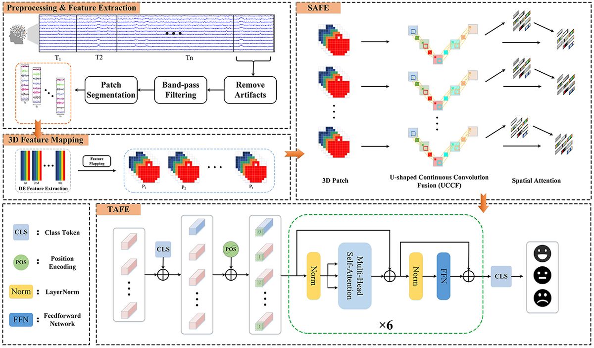
2 Methods

In this section, we introduce the methods and the Hybrid Attention Spatio-Temporal Feature Fusion Network (HASTF) proposed in this paper. As shown in Figure 1, the overall framework can be divided into four parts: Preprocessing & Feature Extraction, 3D Feature Mapping, Spatial Attention Feature Extractor (SAFE) and Temporal Attention Feature Extractor (TAFE). Each part will be introduced in detail below.

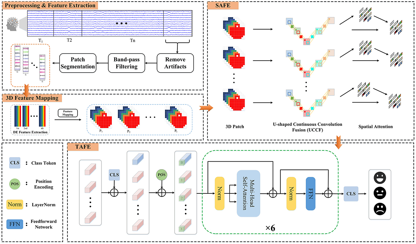
Figure 1. The framework diagram of the hybrid attention spatio-temporal feature fusion network (HASTF) for EEG emotion recognition.

2.1 Preprocessing and feature extraction

For the preprocessed EEG signal X ∈ ℝ(C×L), where C represents the number of EEG channels and L is the EEG sampling time. According to Cai et al. (2024) and Yi et al. (2024), EEG contains various frequency components, which are associated with different functional states of the brain. Therefore, we first use a third-order Butterworth bandpass filter to decomposed the signal into Delta (1–4 Hz), Theta (4–8 Hz), Alpha (8–13 Hz), Beta (13–31 Hz), and Gamma (31–50 Hz), which can be described as Equation 1. This ensures a smooth transition at frequency boundaries and effective separation.

{yDelta=butter_pass(1,4)yTheta=butter_pass(4,8)yAlpha=butter_pass(8,13)yBeta=butter_pass(13,31)yGamma=butter_pass(31,50)    (1)

Then, the signal is non-overlappingly segmented into n time windows of length T. In this study, T is set to 8 s for the DEAP dataset and 11 s for the SEED dataset. Each time window is further divided into smaller patches of 1-s length. For each patch, DE features are extracted in the five frequency bands according to the following formula:

DE(X)=∫-∞∞f(x)logf(x)dx    (2)

Since the EEG signals within each subband tend to closely approximate a Gaussian distribution, f(x) can be written as f(x)=12πσ2exp(-(x-μ)22σ2). Where μ and σ2 represent the expectation and variance of X, respectively. Therefore, the result of the above formula is

DE(X)=12log(2πeσ2)    (3)

Here, e is the base of the natural logarithm.

2.2 3D feature mapping

After calculating the DE characteristics of each frequency band, we process the EEG data into patches one by one. Each patch P ∈ ℝ(n×T×B×C), where n is the number of time windows, T is the number of patches in each time window, B is the number of frequency bands, here B = 5, C is the number of channels. When collecting EEG, electrode caps that comply with the international 10-20 standard are used for data collection. What we want is to restore the arrangement of electrodes on the brain and integrate frequency, spatial and temporal characteristics. Specifically, we arrange the electrode channels in a 2D matrix format that preserves their relative positions as they are placed on the scalp (Yang et al., 2018a; Shen et al., 2020; Xiao et al., 2022). Figure 2 is the mapping diagram of 32 and 62 electrode channels.

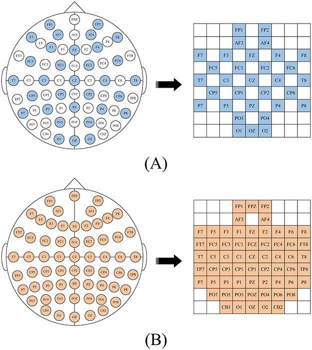
Figure 2. 2D mapping of (A) DEAP dataset, (B) SEED dataset.

2.3 Spatial attention feature extractor

The role of the Spatial Attention Feature Extractor (SAFE) is to extract spatial features from the EEG data to adaptively capture the most crucial EEG channels within the 3D patch. As shown in Figure 3. It primarily consists of two parts, namely the U-shaped Continuous Convolution Fusion module (UCCF) and the parameter-free Spatial Attention Module (SA). And we provided detailed explanations for the research motivation behind each module and their specific details.

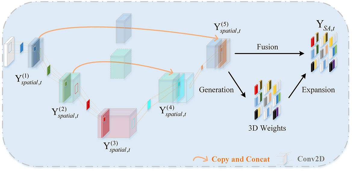
Figure 3. The framework diagram of the SAFE.

2.3.1 U-shaped continuous convolution fusion module

Due to the relatively small dimensions (9 × 9) of the 3D features after 3D mapping, applying conventional convolution operations as used in image processing directly would result in an excessively large receptive field. Such approaches have failed to capture enough fine-grained features (Dumoulin and Visin, 2016; O'shea and Nash, 2015). There could be two potential solutions to this problem. The first involves using shallow networks with small kernel sizes, which is unsatisfactory in terms of capturing spatial features (Tan and Le, 2019). The other one is to employ a deeper network, but this could lead to issues such as overfitting and gradient explosion (Fan et al., 2024). For images, adjacent pixels often exhibit minimal differences, so researchers do not need to excessively emphasize fine-grained features when processing images. while the 3D EEG features are distinct, each “pixel” represents an individual channel, and the relationships between channels are subtle and intricate. Despite the secondary processing of channels based on electrode placement, some neighboring electrodes may have weak relationships, while some distant electrodes may have strong connections (Jin et al., 2024). So, we need to focus more on the fine-grained features of the entire 3D patch. Skip connections (Ronneberger et al., 2015) is introduced into the network, as shown in Figure 3. There are two branches, the “channel expansion” branch on the left and the “channel contraction” branch on the right. These two branches are connected via a cascade operation. It is worth noting that, in the corresponding layers of the two branches, there is a fusion of intermediate features, creating skip connections. This approach ensures that the network can capture sufficient fine-grained features while mitigating overfitting to some extent.

In previous sections, we rearranged the DE features to obtain 3D patches. The input data for UCCF is represented as Xt∈ℝ(n×B×h×w), where n is the number of windows, B is the number of frequency bands, h and w are the length and width of the two-dimensional feature matrix, respectively. The three-dimensional structure of the EEG patches integrate spatial features, frequency band features and time features to facilitate network extraction and processing. Specifically, the structure of each patch is Pi = (x1, 1, x1, 2, …, xh, w), where xi,j∈ℝ(h×w). Let Yspatial,t(k) represent the output of the k-th layer spatial convolution, Yspatial,t(k)∈ℝ(n×Bk×hk×wk), where Bk, hk, wk represent the number, length and width of feature maps obtained as the output of the k-th layer. Yspatial,t(k) can be defined as:

Yspatial,t(k)=ΦReLU(Conv2D(Yspatial,t(k-1),S(k)))    (4)

Where Sk is the kernel size of the k-th convolutional layer. Yspatial,t(k-1) represents the output of the previous layer. Conv2D(.) represents a two-dimensional convolution operation. ΦReIU(.) is RELU activation function. Due to the existence of skip connections, the spatial convolution output formulas for the 4th and 5th layers are different, defined as follows:

Yspatial,t(4)=ΦReLU(Conv2D(CAT(Yspatial,t(3),Yspatial,t(2)),S(4)))    (5) Yspatial,t(5)=ΦReLU(Conv2D(CAT(Yspatial,t(4),Yspatial,t(1)),S(5)))    (6)

Where CAT(A, B) represents the concatenation operation, meaning A and B are joined along a certain dimension to form a new vector, which is then used as a new input and passed through the corresponding spatial convolutional layer.

2.3.2 Spatial attention

The EEG signal is essentially a bioelectrical signal, and its generation is related to the neural mechanism of the human brain. When a neuron becomes active, it often leads to a spatial inhibition in the surrounding area to suppress neighboring neurons (Yang et al., 2021). Therefore, neurons that exhibit this inhibitory effect on their surroundings are relatively expected to have higher weights. Our attention module, based on this theory, employs a parameter-free method to directly compute the attention weights for 3D inputs. The specific approach is as follows:

To estimate the importance of each individual neuron, based on the spatial inhibition phenomenon, a straightforward approach is to measure the linear separability between the target neuron and other neurons. Based on linear separability theory, let et denote the energy of neuron t, establish the energy equation as follows:

et(wt,bt,y,xi)=(yt-t^)2+1M-1∑i=1M-1(yo-x^i)2    (7)

where t^=wtt+bt and x^i=wtxi+bt are the linear transformations of xi and t, respectively. And t is the target neuron for which the degree of correlation needs to be calculated and xi represents other neurons except t, i represents the neuron index, wt and bt are the weight coefficients and bias coefficients in linear transformation. M represents the total number of channels in a specific frequency band. When t^ equals yt and xi^ equals y0, this formula can obtain the minimum value, which is equivalent to finding the linear separability between the target neuron t^ and other neurons xi^. In order to facilitate calculation, the two constants yo and yt are set to −1 and 1, respectively. 0 can be rewritten as

et(wt,bt,y,xi)=1M-1∑i=1M-1(-1-(wtxi+bt))2       +(1-(wtt+bt))2+λwt2    (8)

where λwt2 is the regularization term, λ is a constant. We can quickly get the analytical solution as:

wt=-2(t-ut)(t-ut)2+2σt2+2λ    (9) bt=-12(t+ut)wt    (10)

Among them, ut=1M-1∑i=1M-1xi, σt2=1M-1∑i=1M-1(xi-ut)2. This is also the condition under which the energy function e attains its minimum value. So, the minimum energy can be obtained as:

et*=4(σ^2+λ)(t-ut)2+2σt2+2λ    (11)

Finally, based on this minimum energy, the importance of each neuron can be quantified, expressed as 1/e*. In order to further adapt the attention mechanism to the attention regulation method in the mammalian brain, gain and scaling are used to enhance features, as shown in Equation 12.

X~=sigmoid(1E)⊙X    (12)

Where X is the original input feature map, and X~ represents the refined feature map after applying the attention module. E represents all neuron nodes, i.e., all EEG channels. sigmoid() The sigmoid function is added to map the values in E to the range of 0–1. Therefore, the spatial attention module can be expressed as:

YSA,t=MP(SA(Yspatial,t))    (13)

where SA(.) represents the spatial attention mechanism module. MP(.) represents max pooling operation. We then perform a flattening operation on the resulting output.

2.4 Temporal attention feature extractor

As shown in Figure 1, the temporal attention feature extractor consists of position encoding embeddings and several identical temporal encoding layers. In each temporal encoding layer, contains multiple self-attention layers, Feedforward Neural Network (FFN) layers, and LayerNorm layers. Additionally, residual connections are applied throughout the network.

After SAFE, the vector already contains spatial feature information. Each vector Yt is treated as an individual token, and these T tokens are combined to form the input sequence for TAFE. In order to capture temporal feature information across the entire sequence, similar to the BERT structure (Devlin et al., 2018), a learnable class token is added at the very beginning of the input sequence to obtain aggregated information from the entire input, i.e.,

Zc=[Yclass,Y1,Y2,…,Yt,…,YT