1 Introduction

Head and neck squamous cell carcinoma (HNSCC) poses a significant global health challenge, ranking as the seventh most prevalent cancer worldwide. It originates in the mucous membranes of the mouth, nose, and throat (1). HNSCC is classified based on its location, encompassing areas like the oral cavity, oropharynx, nasal cavity, paranasal sinuses, nasopharynx, larynx, and hypopharynx. Depending on the site of origin, it may present as abnormal patches, open sores, bleeding, pain, sinus congestion, sore throat, earache, difficulty swallowing, hoarse voice, breathing difficulties, or lymph node enlargement. HNSCC has the potential to metastasize to other parts of the body, contributing to over 800,000 new cancer diagnoses annually (2, 3).

Radiotherapy is integral to HNSCC treatment. The conventional approach involves administering 2 Gy doses daily on weekdays, accumulating to a total of 70 Gy, with a focus on the primary tumor and affected lymph nodes. Recent decades have seen significant technological advancements, especially with the adoption of intensity-modulated radiotherapy (IMRT). This innovation enables precise delivery of high-dose radiation to the tumor, minimizing exposure to surrounding healthy tissues. The evolution in technology significantly reduces both immediate and delayed toxicity associated with the treatment.

However, treating HNSCC with radiotherapy is still challenging due to several factors (4–7). The intricate anatomy of the head and neck, coupled with its proximity to critical structures, poses challenges in delivering high doses of radiation without significant side effects. Radiation-induced side effects can substantially impact a patient’s quality of life, and adherence to conventional fractionation schedules can be challenging, particularly for those with limited resources. Factors such as comorbidities, substance use, and underinsurance further complicate the treatment landscape. Timely completion is crucial, but obstacles like transportation, lack of caregiver support, and financial strain may hinder adherence. The aging HNSCC population faces additional challenges, given their increased susceptibility to severe toxicity. Addressing these challenges could offer benefits by reducing the burden and duration of radiation therapy, making it more logistically feasible without compromising efficacy.

HNSCC tumors testing negative for Human Papillomavirus (HPV) can demonstrate rapid growth and resistance to radiation therapy. HPV is a group of more than 200 related viruses, with several types linked to cancer development, particularly in the genital and oropharyngeal regions (8). HPV-negative cancers, often associated with tobacco and alcohol use, tend to be more aggressive and less responsive to treatment, with recurrence rates exceeding 35% for advanced stages (9). Despite treatment advancements, cancer recurrence remains a major issue, with a locoregional recurrence rate of 15–50%. While salvage surgery may offer a curative option for patients with resectable locoregional recurrence, it is often not feasible or only possible with severe complications and limited success rates. Furthermore, advanced and recurrent cancers often develop resistance to treatment, making them more challenging to manage (10).

These factors necessitate ongoing research for more effective, less toxic, and logistically simplified HNSCC radiotherapy strategies (11). Radiobiological modeling is important for achieving these goals (12). The clinical utility of the linear-quadratic (LQ) model lies in its ability to compare fractionation schedules and predict radiation responses. In this model, tumor sensitivity to dose per fraction is governed by the α/β ratio. For HNSCC the α/β ratio is relatively high (around 10 Gy), suggesting that its sensitivity to large doses per fraction is not as large as for some cancers (e.g. breast and prostate) with smaller α/β ratios. For this reason, hypofractionation involving doses per fraction >2 Gy was not as thoroughly investigated for HNSCC as for these other cancers, and was mainly used with palliative rather than curative intent for HNSCC. Instead, many HNSCC clinical trials have investigated the opposite approach of hyperfractionation with smaller fractions twice or three times daily to exploit the radiobiological distinction between tumor and normal tissue (13). The administration of small fractions twice per day decreases the incidence of late toxicity, enabling the delivery of higher total radiation doses compared to conventional dosing. Another alternative - accelerated radiotherapy - addresses tumor repopulation concerns by delivering doses of 1.8–2 Gy twice daily or more than five fractions per week, thereby reducing the overall treatment time (12). The reduction in overall treatment time serves to mitigate tumor repopulation. Both strategies have the potential to enhance tumor control.

To address these challenges comprehensively, we adopt a sequential machine learning approach. Initially, we employ Random Survival Forests (RSF) to broadly analyze survival data and identify significant predictors of outcomes. This is followed by a targeted causal investigation using Causal Survival Forests (CSF), which allows us to delve deeper into the causal relationships between treatment variables and patient survival. This pipeline approach ensures a thorough exploration of the data, starting with general pattern identification and leading to specific causal inferences.

Several randomized trials have investigated various radiotherapy schedules for head and neck cancer, but conflicting results regarding tumor control and survival have emerged. The inconsistency is mainly attributed to trial heterogeneity and small sample sizes. Despite these challenges, the trials suggest that modifications in fractionation are often linked to more frequent acute side effects, while late toxicity rates are similar or less frequent compared to conventional fractionation radiotherapy.

The Meta-Analysis of Radiotherapy in Carcinomas of Head and Neck (MARCH) revealed that altered fractionation radiotherapy is associated with improved overall survival and progression-free survival when compared to conventional fractionation radiotherapy (13). The analyzed trials were categorized based on specific altered fractionation techniques. These categories included hyperfractionation, involving a higher total dose administered through twice-daily fractions within the same overall treatment time; moderate acceleration, maintaining an unchanged total dose but delivered more expeditiously (typically about 1 week faster); and very accelerated radiotherapy with dose reduction, reducing the duration by 50% or more, accompanied by a total dose decrease of approximately 15%. The meta-analysis notably excluded trials investigating hypofractionated radiotherapy, primarily used in palliative cases with doses per fraction >2.5 Gy. This comprehensive analysis affirmed the effectiveness of altered fractionation radiotherapy, especially hyperfractionation, over conventional fractionation radiotherapy.

However, hyperfractionation imposes a logistical challenge which can result in reduced compliance with the therapy. Hypofractionation using fewer larger fractions delivered over a shorter overall time alleviates this issue, and the shortened treatment time is useful to counteract repopulation of quickly growing HNSCC tumors. Navigating the radiobiological complexities of hypofractionation, where the delicate balance between tumor control and toxicity is crucial, represents a key consideration (7). The adoption of accelerated regimens hinges on mucosal tolerance, with hypofractionation demonstrating feasibility when considering mucosal tolerance, resulting in shorter acute side effects and improved tolerability. Initiatives transitioning from conventional to hypofractionation must carefully weigh the impact on late toxicity. While shorter regimens may mitigate late effects, the heightened radiosensitivity of tissues during prolonged radiation courses poses challenges. Studies comparing 3 and 5 weeks of radiation therapy for HNSCC show varied outcomes in tumor control and late toxicity. Successful implementation of hypofractionation in HNSCC treatment requires a comprehensive approach incorporating modern techniques, systemic therapy, and vigilant monitoring.

Importantly, there has been little progress for HPV-negative HNSCCs in the past two decades (7). Despite efforts to explore systemic therapies beyond cisplatin, achieving better disease control remains challenging. However, potential advancements are anticipated with emerging agents and adjuvant therapies. Hypofractionation, endorsed through noninferiority trials across various cancers, has become a preferred practice in multiple disease sites, enhancing treatment efficiency and reducing costs. The ongoing investigation into ultrahypofractionation (≤5 fractions) represents a second wave of studies aiming to further optimize treatment approaches.

Amidst ongoing HNSCC clinical trials, such as HEADLIGHT (Mayo Clinic), NCT05075980; NCT04284540 (Mount Sinai); HYPORT (NCT04403620), HYHOPE (NCT04580446) at the University of Texas Southwestern; and DEHART (NCT04477759), HART-HN (NCT 05120947), HyPR-HN (NCT05538533) at the Medical College of Wisconsin, there is a discernible interest in adopting hypofractionation for head and neck cancer. While hypofractionation is already applied in specific cases, such as early-stage glottic cancer, stereotactic body radiation therapy for reirradiation, palliation, and heavy ion therapy, it is not universally applicable for all head and neck cancers. Existing uncertainties, such as the absence of late toxicity assessments beyond 5 years in ongoing studies and limited randomized comparisons with conventional fractionation, underscore the need for a cautious approach. Some trials employ a time-to-event continuous reassessment methodology (TiTE-CRM), an adaptive statistical approach, to assess delayed toxicity. Key considerations include the safety of delivering radiosensitizing cisplatin with hypofractionation, economic implications, and the generalizability of findings beyond specialty centers. The ongoing exploration of conformal hypofractionation should prompt a comprehensive evaluation of its potential benefits for patients with HNSCCs.

Our previous analyses (14, 15) of classic radiotherapy-only HNSCC clinical trials data using mechanistically-motivated quantitative models of tumor repopulation and killing by radiotherapy predicted that hypofractionation involving increased doses/fraction and reduced overall treatment durations, or hyperfractionation with twice-daily fractions, improve tumor control and reduces late normal tissue toxicity, compared with protocols using 35x2 Gy fractions spread over 7 weeks. Specifically, in the first study (16) we explored an alternative dose-dependent (DD) model of accelerated tumor repopulation (AR), where the onset time and rate of AR depend on the number of tumor clonogens killed, thus on radiation dose and dose-fractionation. This model produced better fits to a wide range of clinical data from HNSCC clinical trials, compared to the standard dose-independent (DI) repopulation model, where the onset time and rate of AR do not depend on radiotherapy details. This model, which assumes that repopulation occurs when a threshold survival fraction is reached, is detailed in the paper by Shuryak et al. (2018) (14). In the second study (17), we performed systematic radiobiological optimization using both DD and DI repopulation models to identify fractionation schemes that improve the balance between tumor control probability (TCP) and long-term normal tissue complication probability (LNTCP).

This research suggested that both hypofractionated schedules with doses >2 Gy/fraction, and twice-daily treatments with <2 Gy/fraction, with reduced overall treatment times, can substantially increase TCP while decreasing LNTCP, compared to a standard 35x2 Gy protocol. This general conclusion applied to both the DI and DD models, although the numerical predictions differed somewhat between models. Hypofractionation and twice-daily hyperfractionation are related in their radiobiological effects because both approaches increase the “intensity” of tumor cell killing per day, and this pattern applies regardless of the details of the repopulation model. Consequently, hypofractionation or its close variant, accelerated hyperfractionation, prove to be efficient strategies in overcoming tumor repopulation, especially in fast-growing tumors like HNSCC.

The main limitations of these modeling studies were: (1) Only classic radiotherapy-alone (no chemotherapy) HNSCC clinical trials were analyzed because the DD and DI models were not developed to handle chemotherapy effects. The treatment approaches and technology implemented in those trials are by now largely outdated. (2) The data were available only in summary form: group averages for different arms of the clinical trials, instead of individual-level patient data. (3) Some important clinical variables such as HPV status were not available.

The objective of the current paper is to scrutinize the validity of the main conclusions of these previous modeling studies about the usefulness of altered radiotherapy fractionation through the lens of contemporary HNSCC patient treatment data, evaluating patients who have undergone modern treatment techniques. To achieve this, we used a comprehensive dataset from the RADCURE project, encompassing records of 3,346 patients treated for head and neck cancer at the University Health Network in Toronto, Canada, from 2005 to 2017 (18, 19). This dataset is particularly valuable due to its extensive coverage of relevant parameters, including radiotherapy dose and fractionation, chemotherapy, various clinical variables, and patient survival outcomes.

We used a two-step analysis approach on the RADCURE data set, which combines mechanistic modeling concepts with state-of-the-art machine learning techniques, beginning with Random Survival Forests (RSF) for an exploratory analysis and followed by Causal Survival Forests (CSF) for a focused causal analysis. This approach is informed by previous work where RSF and Shapley Additive Explanations were effectively employed to model nonlinear relationships in radiation exposure studies. This study aims to thoroughly investigate the effects of radiotherapy fractionation on overall patient survival (OS) and cause-specific mortality (deaths from the index cancer, other cancers or other non-cancer causes), contributing valuable insights to the ongoing discourse on optimizing head and neck cancer treatment strategies.

Importantly, conventional statistical and machine learning approaches primarily emphasize prediction based on variable correlations (20). These methods produce associations rather than causation regarding the influence of individual features (e.g., radiation dose). In contrast, Causal Machine Learning (CML), such as causal survival forests (CSF), can be used for establishing causal relationships between variables, facilitating the generalization of results across various scenarios and enabling targeted interventions (20–23).

Predictive and causal modeling approaches are fundamentally distinct (20, 24–26). In predictive tasks, the objective is to accurately predict an outcome variable, such as patient survival time, based on predictor variables (features). The accuracy of these predictions for new datasets depends on the resemblance of data distributions and correlation structures to the initial training data. In contrast, causal analysis involves modeling how changes in a specific feature, such as radiation exposure, influence the outcome. Causal modeling’s utility extends beyond the distributions of training data, making it adaptable to various datasets, even with disparate variable correlations. This distinction highlights that predictive modeling is an unreliable approach for causal inference, especially in observational data. Predictive models tackle associations, while causal models explore interventions and counterfactuals, assessing the effects of modifying causal variables (20). Maximizing prediction accuracy during training may introduce biases, such as collider bias and overcontrol bias, which can potentially lead to errors in causal inference (27–30). Common techniques used in predictive modeling, like regularization and feature selection, may also yield inaccurate causal inferences. Predictive models can only be causally interpreted when the feature of interest is independent not only of other features but also of unobserved confounders.

In contrast, CML methods are explicitly designed to model cause-and-effect relationships, even within complex data featuring confounders. CML is not constrained by strict assumptions about the shapes of causal relationships. Its main assumptions include the stability of cause-and-effect relationships, the absence of reverse causation, ignorability, and positivity. The ignorability assumption posits the absence of unmeasured confounding variables affecting both the treatment variable (the focal variable for causal investigation) and the outcome variable (the variable under causal scrutiny). Essentially, it presumes that all relevant confounding variables are both measured and considered in the analysis. While ignorability is not directly assessable, refutation methods can indirectly evaluate it. Positivity assumes that the likelihood of receiving a particular treatment level (exposure) exceeds zero for all strata of covariates (confounding variables). This implies that every subgroup within the population has a nonzero chance of being exposed to the treatment of interest. Failing to meet the positivity assumption can make estimating causal effects challenging, as there may be groups where the treatment is never observed, rendering it impossible to assess its impact within those groups.

Another very important capability of several CML methods is the doubly robust estimator property. A doubly robust estimator (DRE) remains unbiased even if either the treatment or outcome model is correctly specified, but not necessarily both. This flexibility enhances the robustness of causal inferences, as it allows for some degree of model misspecification without compromising the reliability of the estimated treatment effects. For example, suppose we are investigating the causal effect of a specific radiotherapy protocol on the survival time of cancer patients. In this scenario, there will be two models: (1) The treatment model, which estimates the effect of radiotherapy on survival time and accounts for various factors, including dose, duration, age, stage of cancer, comorbidities and other patient characteristics. (2) The outcome model, which predicts patient survival time and considers the same relevant variables as the first model. The DRE property implies that even if only one of these two models (but not both) is correctly specified, the estimated causal effect of the radiotherapy remains unbiased. This robustness is valuable because, in practice, it is very challenging to perfectly specify both models due to the complexity of medical scenarios and the presence of unobserved variables. Thus, the DRE property ensures that causal inferences remain reliable and unbiased even when there is some degree of uncertainty or misspecification in the models used to estimate treatment effects and predict outcomes.

While CML methods have been gaining recognition in a range of disciplines (22, 23, 31, 32), their adoption in radiation oncology so far remains limited. CML offers a more thorough and accurate comprehension of these relationships, with the capacity to estimate effects at both population and individual levels, holding substantial potential for informing radiation oncology decision-making.

In this study, we combined the strengths of three types of radiobiological modeling joined into a coherent analysis pipeline: (1) The mechanistic concept of biologically effective dose (BED) was implemented for the standard dose-independent (DI) tumor repopulation model, for our alternative dose-dependent (DD) repopulation model, and for a simple model with no repopulation (BEDsimp). (2) A powerful predictive machine learning algorithm - random survival forests (RSF) – was employed as an initial step to model patient overall survival (OS) and cause-specific mortality (deaths from the index cancer, other cancers or other non-cancer causes) using the BED variants together with clinical variables. (3) Targeted causal inference analyses were then performed using the CSF algorithm to estimate the causal effect of each BED variant separately on OS. We believe that the results of these analyses deepen the current insights into how radiotherapy fractionation affects the effectiveness of HNSCC treatment.

2 Materials and methods

A detailed description of the data processing and machine learning analyses is provided in Supplementary Methods in the Supplementary Materials. The main aspects are provided below.

2.1 Data collection

The dataset was obtained from the RADCURE project, consisting of 3,346 head and neck cancer patients treated with definitive radiotherapy (RT) at the University Health Network in Toronto, Canada (18, 19). This dataset is very useful for investigating the effects of different radiotherapy fractionation schemes on HNSCC patient survival because it includes a variety of total doses and doses per fraction. To provide a comprehensive overview of the treatment regimens used in the dataset, we analyzed the distribution of different fractionation schedules. Table 1 summarizes the number of patients treated with various numbers of fractions and doses per fraction. It shows that while most patients were (expectedly) treated with the standard 35 fraction/70 Gy regimen, 4 other regimens were represented by >50 patients each, indicating the diversity of the RADCURE data set.

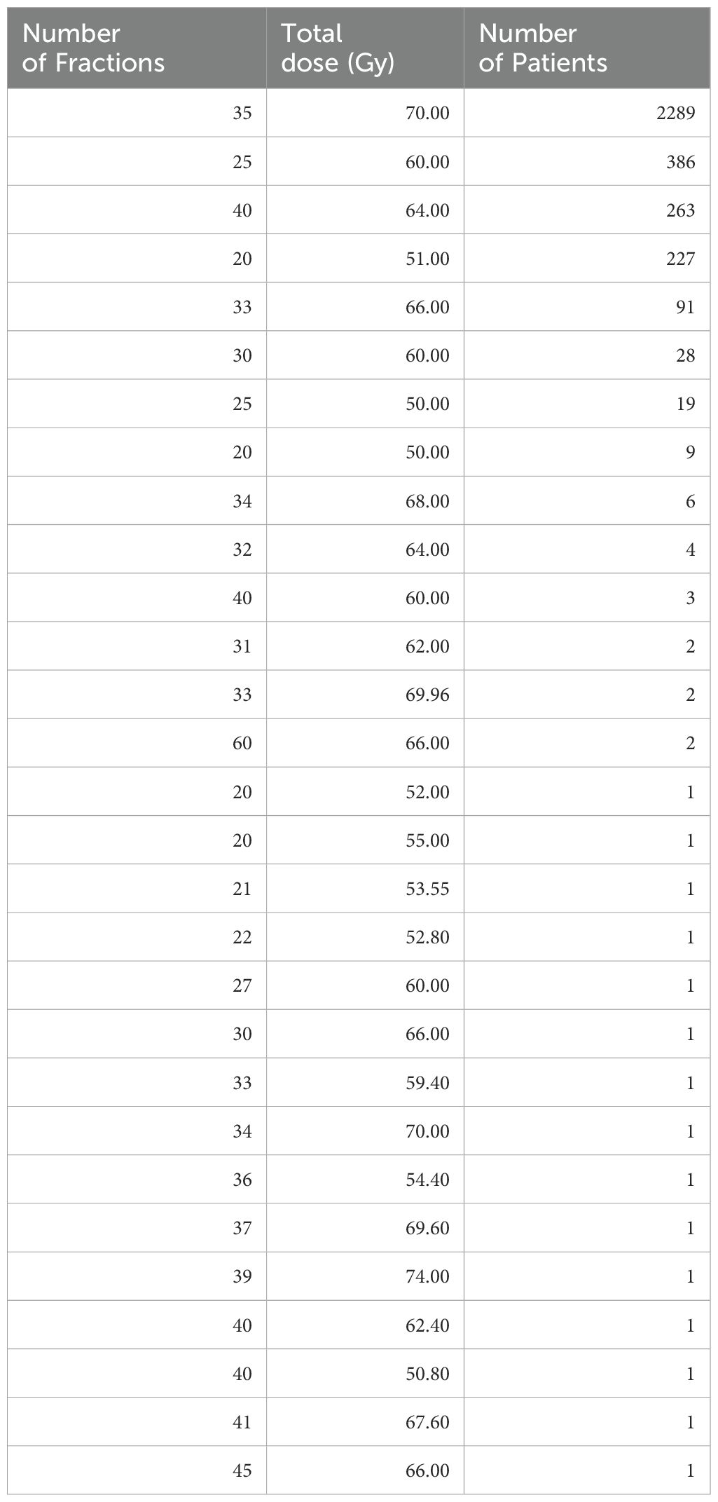
Table 1. Detailed breakdown of radiotherapy fractionation schedules in the RADCURE data set.

2.2 Data preprocessing and feature selection

The RADCURE data set contained numerous clinical variables, and for analysis we selected the following most relevant ones, trying to avoid redundancy: Age (patient age, years), Sex (0=female, 1=male), SmokingPY (number of packs smoked in a year), Stagenumeric (AJCC 7th edition staging categories, converted into integers of 0–4), HPV (tumor HPV status determined by p16 IHC ;+/- HPV DNA by PCR), Chemo (1=received concurrent chemoradiotherapy, 0=did not receive concurrent chemoradiotherapy), RTyear (calendar year of the radiotherapy treatment), Status (binary indicator of vital status at last contact date), LengthFU (duration of follow up from diagnosis to last contact date in years). The HPV status was categorical, indicating positive, negative, or unknown (missing). To incorporate this information into our analysis, we applied one-hot encoding, representing HPV- as the default, while creating separate binary columns for HPVPositive and HPVUnknown. The Status and LengthFU variables were the outcome variables, indicating overall survival (OS). The data were imported and analyzed using the R and Python programming languages.

In addition to studying OS, we performed a targeted analysis of cause-specific mortality in HNSCC patients, distinguishing deaths from the index cancer, other cancers or other (non-cancer) causes. In this analysis we also assessed the contributions of head and neck cancer diagnosis site to each cause of death. We selected only those sites which contained data for ≥20 patients each (Esophagus, Hypopharynx, Larynx, Lip Oral Cavity, Nasal Cavity, Oropharynx), and discarded sites with smaller numbers of patients and entries with unknown diagnosis site. This data subset contained 2,651 patients. These selection criteria were designed to exclude those diagnosis sites for which too few samples were available to be informative. The different diagnoses sites were coded as separate columns of binary (0 or 1) variables, with 1 indicating that the given sample had the tumor at the given site.

2.3 Calculation of biologically effective dose for different tumor killing and repopulation models

To compare the effects of various radiotherapy regimens present in the RADCURE data set, we employed the well-established Biologically Effective Dose (BED) concept (33). If tumor repopulation is neglected, a simplistic BED can be calculated as follows, where m is the number of fractions, d is dose per fraction, and r is the α/β ratio (assumed to be 10 Gy for HNSCC):

A more advanced BED version which includes accelerated tumor repopulation (AR) which is assumed to begin at a fixed onset time Tk is based on the work of Withers et al (34). Since Tk is assumed to be independent of radiotherapy details such as dose or dose/fraction, we called this the “dose independent” (DI) model, and the consequent BED is labeled BEDDI. Based on our previous publication (14), the equation for BEDDI is as follows, where λ = accelerated tumor repopulation rate, g = background slow repopulation rate (not accelerated), Tk = onset time for accelerated repopulation, T = total radiotherapy treatment time:

BEDDI=[m α dd + rr− g T − λ max(0, T − Tk)]/α

As another alternative, we considered our proposed “dose dependent” (DD) tumor repopulation model, where both the onset time and rate of AR are assumed to depend on the average fraction of tumor cells killed by radiotherapy each day (14). In other words, in this model the tumor responds to a higher “intensity” of tumor cell killing by radiotherapy by starting AR earlier and increasing its rate. AR is assumed to begin when the natural logarithm of the tumor cell surviving fraction drops below a certain value –C. The equation describing BEDDD from this model is below:

BEDDD=[r λ(exp(−m α dd + rT r)− 1)max(0, −T−m α d (d + r)+ C rm α d (d + r))+ (α d m − T g) r + m α d2]r α

Details of the derivations of BEDDI and BEDDD are described in the Supplementary Methods. The parameters were taken from reference (14). They were as follows: BEDDI: α = 0.069 Gy-1, λ = 0.035 days-1, Tk = 28.6 days; BEDDD: α = 0.224 Gy-1, λ = 1.17 days-1, C = 14.5. The default α/β ratio r was 10 Gy for both models (14). The resulting BEDsimp, BEDDI and BEDDD variables were included in the RADCURE data set as predictors of OS. These parameter values were derived from fitting the DD and DI models to a collection of classical HNSCC clinical trials involving different radiotherapy fractionation schemes.

Since it is known that the α/β ratio for HNSCC can vary considerably among different studies and data sets (35), in the subset analysis described above for cause-specific mortality we also assessed sensitivity of model predictions to this parameter by including in the model different versions of BEDsimp, BEDDI and BEDDD which differed from each other by using different α/β values, 7, 10 or 13 Gy. These variables were labeled with extra subscripts, e.g. BEDDD 7, BEDDD 10 and BEDDD 13.

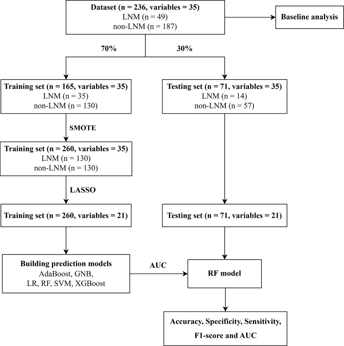
2.4 Machine learning pipeline for predictive and causal analysis

Our study utilizes a unified two-step machine learning pipeline to analyze the effects of radiotherapy fractionation on overall survival. In the first step, we employ Random Survival Forests (RSF) to conduct a general analysis of the dataset, leveraging RSF’s capability to handle censored data and capture complex interactions between features. This exploratory phase helps in identifying significant predictors of patient outcomes and sets the stage for a more detailed investigation. The second step involves deploying Causal Survival Forests (CSF) to specifically explore the causal impact of identified variables on survival. This targeted approach allows us to substantiate the patterns observed in the RSF analysis with a causal perspective, providing insights into how changes in treatment variables could potentially affect patient survival. This sequential utilization of RSF and CSF underscores our comprehensive strategy to not only predict survival outcomes but to understand the underlying causal mechanisms. In each analysis, the data set was randomly divided (70:30) into training and testing portions, with all model fitting and optimization being performed on the training portion and the testing portion being withheld for evaluation. The two steps of this approach are described below.

Step 1: Predictive Machine Learning Analysis using Random Survival Forests (RSF).

We utilized Random Survival Forest (RSF), a predictive machine learning method, to model OS using all the other available variables (features) in the data set. The goals of this analysis were to identify: (1) How accurately can OS be predicted using the available variables? (2) Which variables are most important contributors to these predictions? (3) How does radiotherapy, represented by the BEDDD, BEDDI and BEDsimp variables, contribute to predicting OS or cause-specific mortality? Separate RSF analyses were performed for all patients in the data set, and separately for the HPV- patients only. SHapley Additive exPlanations (SHAP) values are a state of the art method for interpreting complex machine learning models, such as those used here. We calculated SHAP values for all features in the RSF model and visualized them. These calculations were implemented using the scikit-survival Python library.

As mentioned above, we also conducted a subset analysis focused on cause-specific mortality, distinguishing deaths from the index cancer, other cancers or other (non-cancer) causes, and evaluating the contribution of diagnosis site and α/β ratio. Since multiple competing causes of death were modeled in this scenario, we used the RSF variant for competing risks, implemented in the randomForestSRC R package (36). The RSF model handles competing risks by simultaneously considering multiple mortality causes. At each node, the model uses a modified log-rank test to choose splits that best separate causes of death. Each terminal node represents data subsets with similar characteristics and predicted outcomes. These competing risk modeling results were visualized using the Cause-Specific Cumulative Hazard Function (CSCHF) and Cumulative Incidence Function (CIF) plots. The CSCHF illustrates the rate of death from a specific event type while considering the presence of other competing events. In contrast, the CIF estimates the marginal probability of death based on its cause-specific probability and overall survival probability. These metrics are vital for comprehending the survival experience involving multiple competing events and offer more interpretable estimates than traditional survival analysis methods. Variable Importance (VIMP) scores, which assess the significance of each feature in predicting outcomes (different mortality causes), were also generated. VIMP is determined by the increase in prediction error when the feature’s values are randomly permuted. A larger increase in prediction error indicates greater importance of the feature. High positive VIMP values signify strong predictive importance.

Step 2: Causal Machine Learning Analysis Using Causal Survival Forest (CSF).

The CSF algorithm, implemented using the causal_survival_forest function of the grf R package (23, 37), was employed to quantify the causal effects of each BED variant (BEDDD, BEDDI or BEDsimp) on OS. The CSF algorithm uses a binary (0 or 1) causal/treatment variable as the input. Consequently, we converted continuous BEDDD, BEDDI or BEDsimp into binary variables by using manually defined cut-points guided by the SHAP analysis results from the RSF model described above. For example, the examination of RSF-generated SHAP values for BEDDD suggested a nonlinear response, where a clear reduction in patient mortality was associated with BEDDD values >61.8 Gy. Consequently, a causal variable for CSF analysis was created where BEDDD values ≤61.8 Gy were mapped to 0, and BEDDD values >61.8 Gy were mapped to 1. The same approach was used to binarize BEDDI and BEDsimp, but with different cutoff values.

Consequently, three separate CSF analyses were performed, using binarized versions of either BEDDD, BEDDI or BEDsimp as the causal/treatment variable. In each case, the other two BED versions were not included in the data set. For example, if binarized BEDDD was the causal variable, BEDDI and BEDsimp were not included. The set of covariates/potential confounders was the same in each analysis: Sex, SmokingPY, Stagenumeric, HPVPositive, HPVUnknown, Chemo, RTyear, Age.

Two estimands (metrics) were selected to describe the causal effect of each BED variant. They were RMST (Restricted Mean Survival Time) and survival probability (SP). RMST represents the average survival time up to a specific time point (e.g., a fixed follow-up time or a certain event occurrence). Notably, it offers a straightforward and easily communicable representation of the average survival duration up to a specified time point. Its significance is particularly pronounced in clinical research, as it provides a clinically comprehensible summary of time-to-event data, facilitating the evaluation of intervention effectiveness and therapeutic outcomes. Additionally, RMST exhibits robustness in the face of violations of the proportional hazards assumption, rendering it well-suited for diverse study scenarios where alternative methods may prove less effective. In comparison, SP refers to the likelihood of an event (death in this case) occurring beyond a given time point. In causal survival forests, SP provides insights into the probability of survival (or event-free survival) at specific time intervals. Both RMST and SP were calculated for various times after treatment. Various sensitivity analyses and refutation tests, described in more detail in Supplementary Methods, were performed to evaluate the robustness of CSF results.

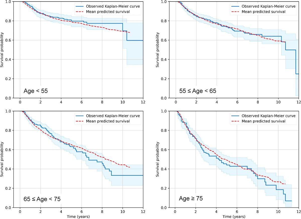
3 Results3.1 Predictive RSF analysis

In the first step of our analysis pipeline, we utilized RSF to explore and predict overall survival (OS) or cause-specific mortality (distinguishing deaths from the index cancer, other cancers or other non-cancer causes) in the RADCCURE patients using the BED variants and clinical variables as features (predictors). Visually, RSF predictions for OS agreed quite well with the observed data: a comparison of mean RSF-predicted and observed Kaplan-Meier survival curves for patients in different age ranges is shown in Figure 1. As expected, OS was reduced for patients of older ages compared with those in younger age groups, and the RSF model captured these patterns adequately. The effects of all other variables were lumped together within each age group, so the plots in Figure 1 are intended only as an overall visualization of model agreement with the data.

Figure 1. Visualization of predictive performance of the RSF model for OS on testing data. Mean predicted Kaplan-Meier survival curves for patients in different age ranges (red dashed curves) are compared with observed patterns (blue solid curves), as function of time after treatment. Blue shaded regions represent 95% confidence intervals for observed survival.

Quantitatively, predictive performance of the RSF algorithm with tuned hyperparameters (min_samples_leaf = 30, min_samples_split = 2, n_estimators = 52) was assessed on training data using 10-fold cross validation (CV), and separately on testing data. On training data (70% of the data set), it generated a mean concordance score (c-index) of 0.759 on training folds and 0.730 on testing folds. On separate testing data (30% of the data set) this model had a c-index of 0.718. Very similar performance was achieved if only BEDDD, rather than all three BED variants (BEDDD, BEDDI and BEDsimp) were included in the model. These results suggest that RSF performance was good, and the model was not overfitting the training data much and was able to generalize well to testing data.

SHAP value summary plots for the RSF model on testing data, which show how different features contributed to the model’s predictions, are displayed in Figures 2A, B. Panels A and B display results for the model variant which included BEDDD, BEDDI and BEDsimp, whereas panels C and D represent the model variant which included only BEDDD (not BEDDI or BEDsimp). In both models, the most important predictors of mortality in this patient population were age, HPV, stage, smoking and calendar year. Chemotherapy was the next most important predictor of mortality. Radiotherapy (BED variants) contributed less than chemotherapy, but still had non-negligible effects. Sex contributed very little to model predictions. These findings suggest that the SHAP contributions of BEDDD and BEDDI are likely to be largely redundant to each other, and it is not necessary to include both of them in the model. BEDsimp contributed less than either BEDDD or BEDDI.

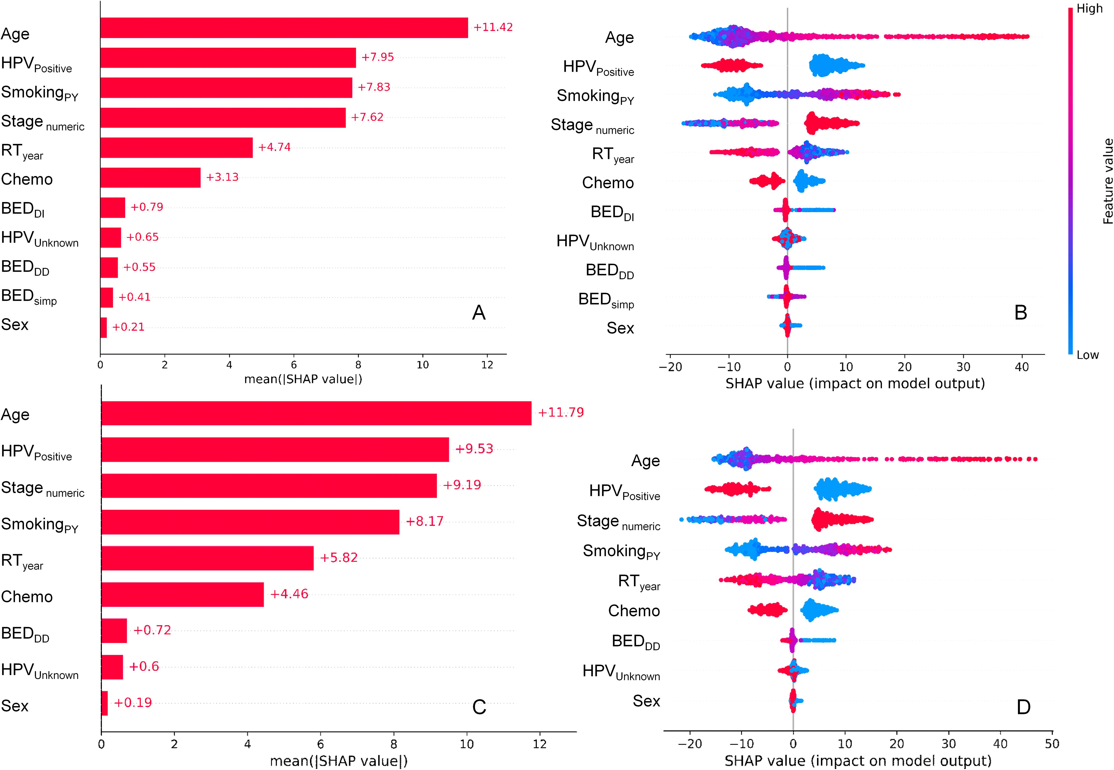
Figure 2. SHAP value summary plots for the RSF model for OS. (A, B) represent the model variant which included BEDDD, BEDDI and BEDsimp, whereas (C, D) represent the model variant which included only BEDDD (not BEDDI or BEDsimp). (A, C) show mean absolute SHAP values for different features, informing abut which features contributed more or less to RSF model predictions. (B, D) show a detailed view where every point is a patient from the testing data set. The SHAP value scale indicates the effect on model predictions: a positive SHAP value implies an increased risk of death, while a negative value implies a reduced risk. The color of the points indicates the value of the feature for that observation, with warm colors representing higher values and cool colors representing lower values.

Figures 2A, C show the mean absolute SHAP values for each feature, whereas Figures 2B, D provide more detail by displaying SHAP values for each individual patient in the testing data set and color coding them by feature value. For example, higher values of age (red points for the Age feature in Figures 2C, D) are associated with high positive SHAP values for Age, indicating that mortality risk is increased at old ages. Conversely, high red values of the HPVPositive feature (which indicate HPV+ patients) were associated with negative SHAP values, indicating that HPV+ status decreased mortality risk. High values of BEDDI or BEDDD were associated with reduced mortality risk, whereas this was not obvious for BEDsimp.

Pearson correlation coefficients between all features and SHAP values in the testing data set are shown in Supplementary Figure 1. BEDDD and BEDDI are strongly correlated with each other and with their SHAP values, whereas the strength of correlation between them and BEDsimp is somewhat weaker. Several other features are also strongly correlated with their own SHAP values, e.g. SmokingPY, Stagenumeric, HPVPositive, Chemo, RTyear, Age.

A more detailed visualization of how the SHAP values of some features of interest are related to the feature values is provided in Figure 3. The y axis in each panel displays normalized SHAP values on a “relative risk” scale, where 1 represents no change from the population average, 1.1 represents a 10% increase in predicted mortality risk, and 0.9 represents a 10% decrease in predicted mortality risk. The SHAP results for BEDDD are shown in Figure 3, and those for BEDDI and BEDsimp from the same model are shown in Supplementary Figure 2.

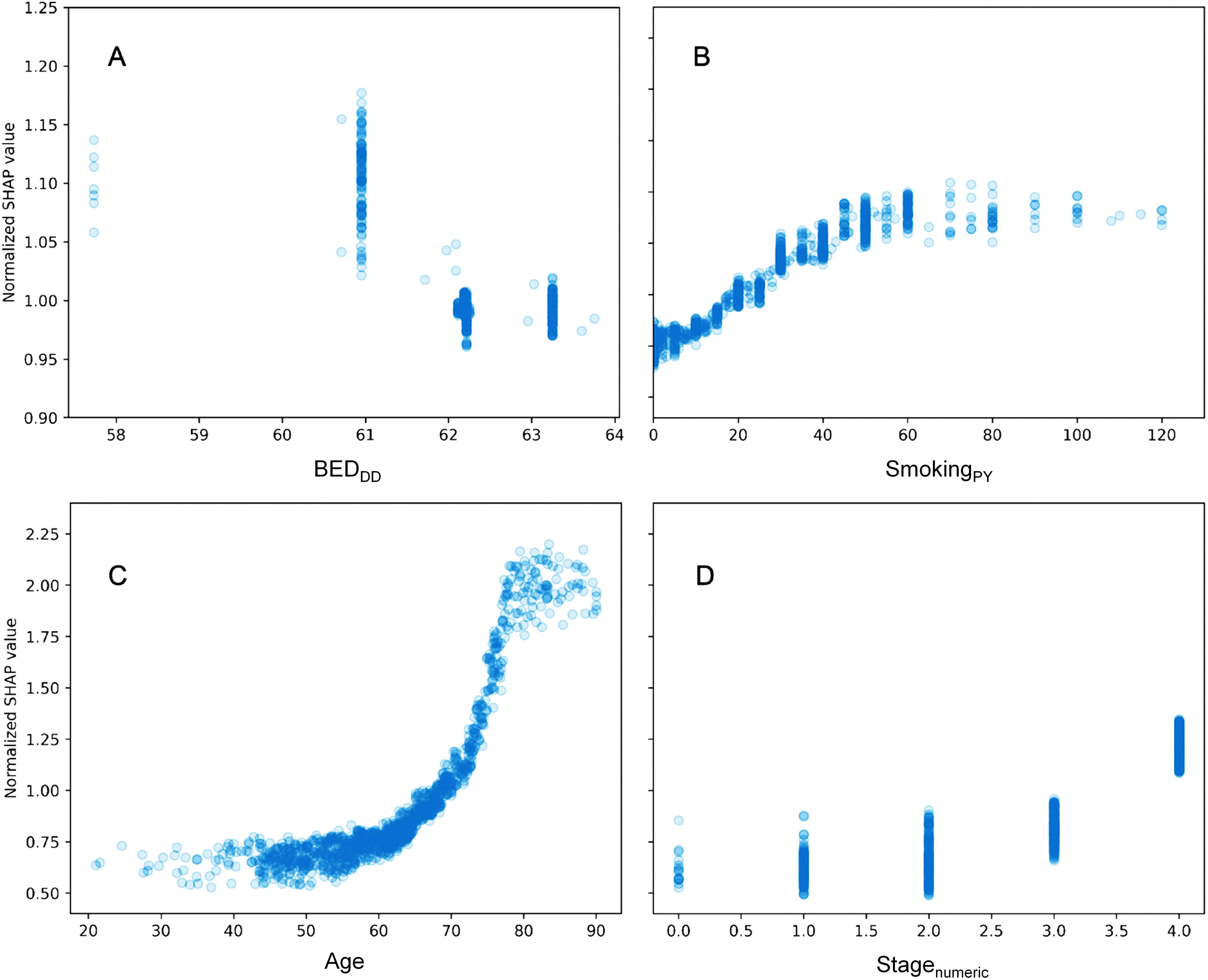
Figure 3. Detailed look at the relationship between some features of interest and their normalized SHAP values in the RSF model. (A) = BEDDD, (B) = SmokingPY, (C) = Age, and (D) = Stagenumeric. The y axis displays normalized SHAP values on a “relative risk” scale, where 1 represents no change from the population average, 1.1 represents a 10% increase in predicted mortality risk, and 0.9 represents a 10% decrease in predicted mortality risk.

For BEDDD and BEDDI the patterns are very similar and nonlinear, suggesting that larger values are associated with reduced mortality. For BEDsimp, however, there is almost no change, suggesting that this BED variant which does not include repopulation is not very useful for predicting mortality. Increasing age, stage and smoking are associated with increased mortality, as expected. Notably, the y axis scales in different panels are different, since age, stage and smoking contributed more to predicting OS in the patient population, compared with the BED variants.

The competing risks RSF analysis for cause-specific mortality, using the optimized number of 300 trees, achieved reasonable concordance scores on both the training (70%) and testing (30%) portions of the analyzed data subset. Specifically, on training data its c-index values were 0.888, 0.936 and 0.863 for deaths from the index cancer, other cancers or other non-cancer causes, respectively. On testing data, its corresponding c-index values were 0.771, 0.810 and 772, respectively. The decrease in performances from training to testing was not dramatic, suggesting a relatively stable model with not much overfitting.

Visualizations of the Cause-Specific Cumulative Hazard Function (CSCHF) and Cumulative Incidence Function (CIF) for this competing risks model revealed different temporal patterns for the different causes of death (Supplementary Figure 3). Most deaths from index cancer (i.e. HNSCC recurrences) occurred within the first 5 years after treatment, whereas death hazards from other cancers and non-cancer diseases continued to increase almost linearly over the entire period of observation.

Examination of Pearson correlation coefficients between variables in this data set (Supplementary Figure 4), particularly between BED variants and CSCHF values for different causes of death 10 years after treatment (Supplementary Table 1), also revealed several interesting findings. For example, BEDsimp variants with different α/β ratios had counterintuitive positive (rather than negative) correlations with death from index cancer. BEDDI variants had negative correlations, as expected, but their values were relatively small, around -0.10. BEDDD variants had stronger negative correlations with death from index cancer, but only for α/β ratios of 7 and 10 Gy, whereas for 13 Gy the correlation switched sign and lost its statistical significance (Supplementary Table 1). Overall, these results suggest that BEDDD and BEDDI have some predictive value for deaths from HNSCC recurrences and perhaps for other causes as well, but (especially for BEDDD) there is some sensitivity to α/β ratios.

Some other variables also had interpretable behavior which conformed to expectations. For example, age was positively correlated with deaths from all causes, especially with non-cancer causes, whereas chemotherapy had expectedly negative correlations with all causes of death (Supplementary Figure 4). There was some variability between correlations among HNSCC diagnosis sites and cause-specific mortality, e.g. positive correlations for hypopharynx and negative ones for oropharynx (Supplementary Figure 4). These findings indicate that hypopharynx tumors were associated with higher mortality, whereas oropharynx tumors were associated with lower mortality.

3.2 RSF analysis of HPV negative patients

The evaluation of the RSF model for the subset of patients with HPV- status was performed as a separate analysis. Predictive performance of the RSF algorithm with tuned hyperparameters (min_samples_leaf = 10, min_samples_split = 2, n_estimators = 65) on this data subset was assessed on training data using 10-fold cross validation (CV), and separately on testing data. On training data, it generated a mean concordance score (c-index) of 0.755 on training folds and 0.634 on testing folds. On separate testing data, this model had a c-index of 0.651. This performance was somewhat worse than on the full data set likely because of reduced sample size: there were only 578 HPV- patients, vs. 3,346 patients in the entire data set.

A more detailed visualization of how the SHAP values of some features of interest are related to the feature values in the HPV- patients only is provided in Figure 4, Supplementary Figure 5. The patterns were generally similar to those found for all patients (Figure 3, Supplementary Figure 2): there was a clear relationship between SHAP values and BEDDD and BEDDI, but not for BEDsimp, and other variables like age, smoking and sex had major contributions. SHAP value summary plots for the RSF model for HPV- patients are shown in Supplementary Figure 6, and a heatmap illustrating the correlation of SHAP values among various clinical factors in the prediction model for HPV- patients is provided in Supplementary Figure 7. In both cases, the patterns were also not very different from those observed for all patients.

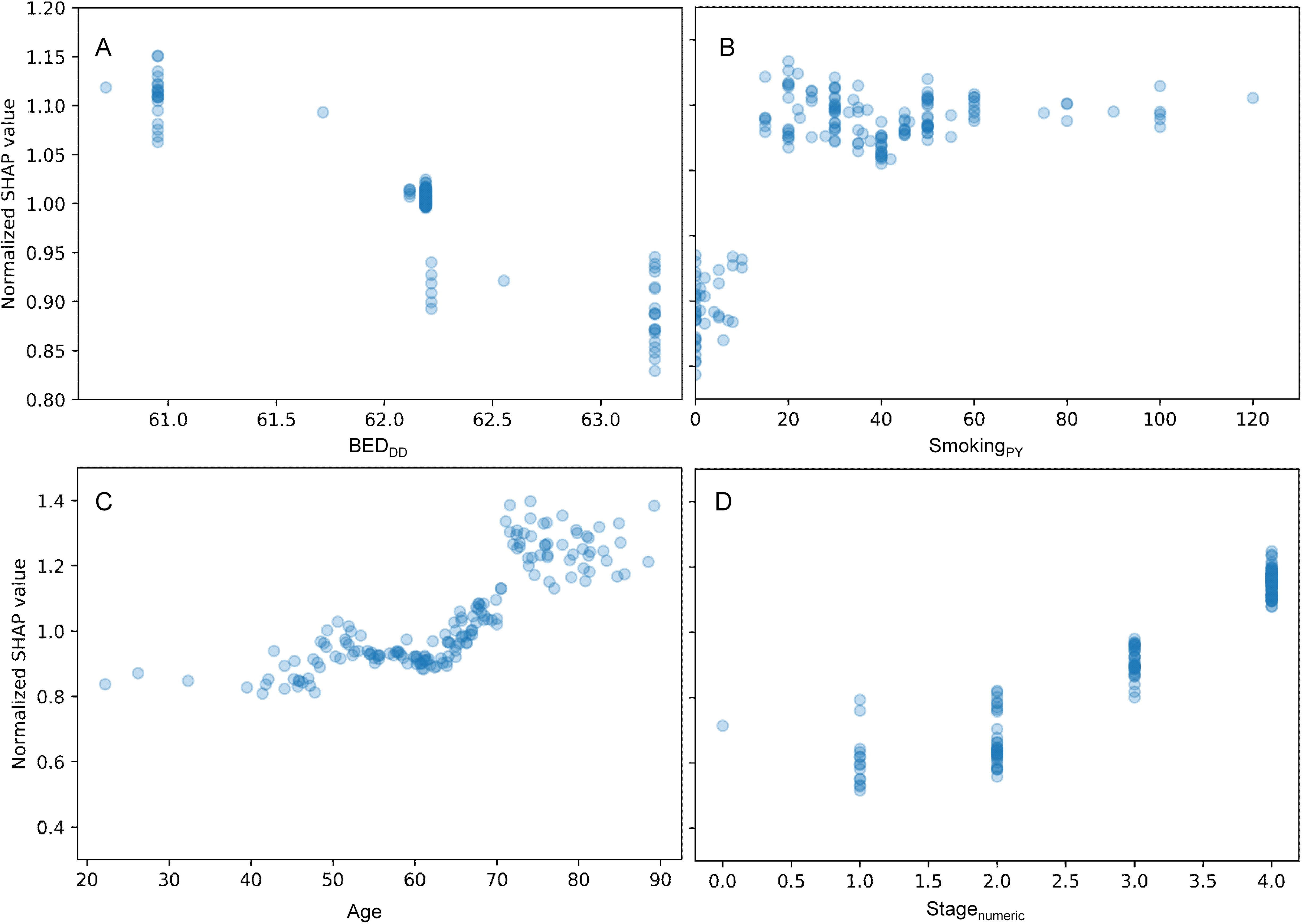
Figure 4. Detailed look at the relationship between some features of interest and their normalized SHAP values for the HPV- patients only. (A) = BEDDD, (B) = SmokingPY, (C) = Age, and (D) = Stagenumeric. The y axis displays normalized SHAP values on a “relative risk” scale, where 1 represents no change from the population average, 1.1 represents a 10% increase in predicted mortality risk, and 0.9 represents a 10% decrease in predicted mortality risk.

3.3 Causal inference CSF analysis

Following the exploratory analysis with RSF, we proceeded to the second step of our pipeline using Causal Survival Forests (CSF). This phase was aimed at conducting a targeted causal analysis, building on the patterns and predictors identified by RSF to delve deeper into their causal relationships with overall survival. Based on the RSF modeling and SHAP value analysis (Figure 3, Supplementary Figure 2), we proceeded to perform targeted causal survival forest (CSF) analyses to look at the causal effects of BEDDD, BEDDI and BEDsimp (one at a time) on OS in this patient population. To perform these analyses, BEDDD was converted into a binary variable by using a manual cut-point of 61.8 Gy, and the same approach was used to binarize BEDDI (with a cut-point of 57.6 Gy) and BEDsimp (70 Gy). The cut-points were selected based on where a clear change in mortality prediction could be seen in the RSF SHAP values (Figure 3, Supplementary Figure 2) for BEDDD and BEDDI. For BEDsimp there was no clear change in the SHAP values as function of feature values, so the 70 Gy cut-point was selected using a similar percentile to the one used to binarize BEDDD and BEDDI.

Figure 5 shows simple univariate comparisons of Kaplan-Meier survival curves for patient groups split by the binarized BEDDD. Supplementary Figure 8 contains similar information for BEDDI and BEDsimp. For the BEDDD and BEDDI variants, the curves were significantly different from each other: logrank test p-value = 3×10-12 for BEDDD and p-value = 1×10-10 for BEDDI. In contrast, there was no significant difference between groups split by BEDsimp (Supplementary Figure 8, p-value = 0.9). If the analysis was restricted to HPV- patients only, there was still a significant difference (p-value 0.01) for BEDDDvs. low BEDDD despite the reduced sample size of the HPV- patient subset.

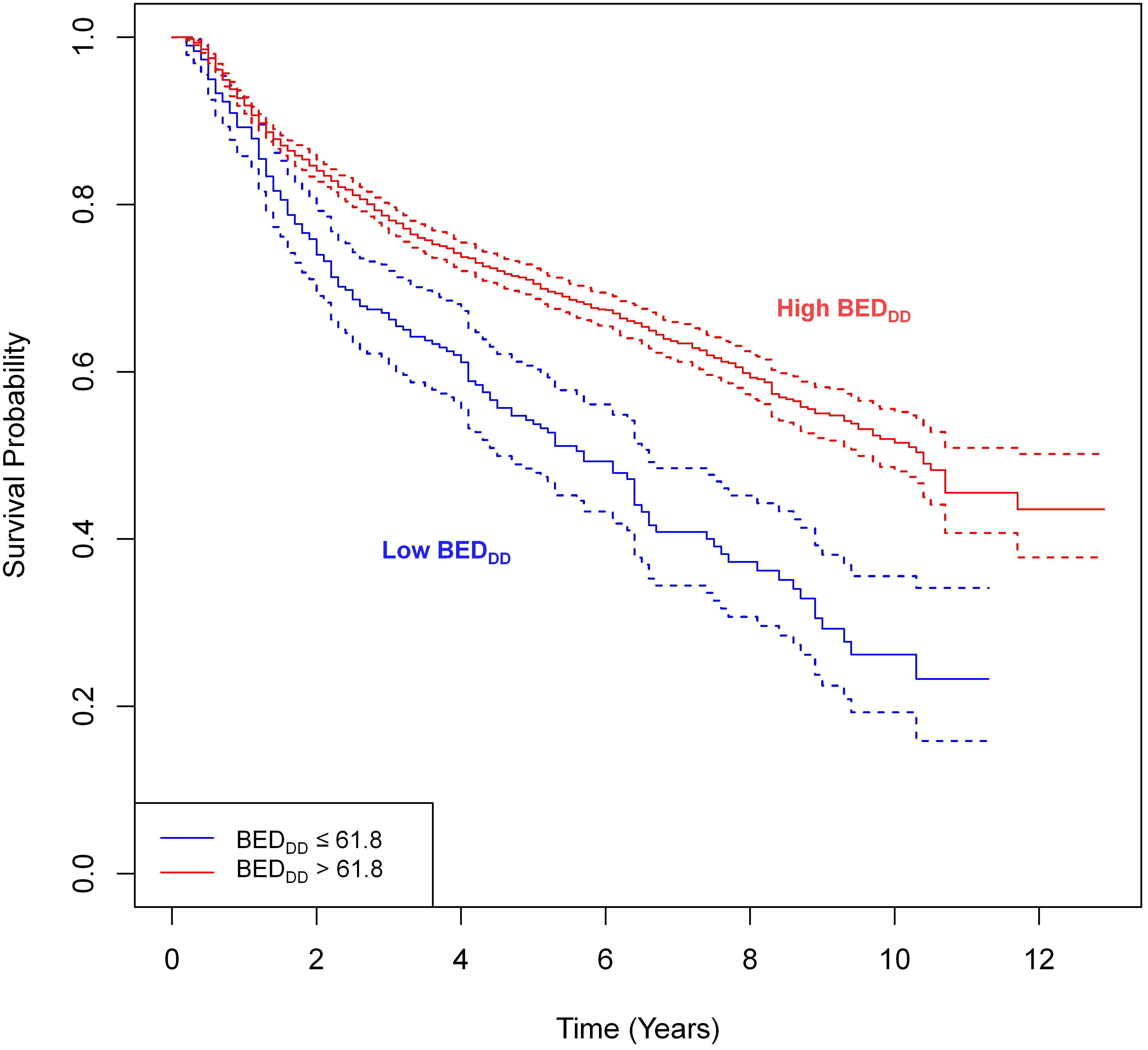
Figure 5. Simple univariate comparisons of Kaplan-Meier survival curves for patient groups based on splitting BEDDD. The splitting cut-points were guided by the SHAP value analysis in the previous figure. The logrank test revealed statistically significant differences between groups: p-value = 3×10-12.

CSF-based causal effect (conditional average treatment effect, CATE) estimates for the effects of binarized BEDDD, BEDDI and BEDsimp on patient OS are shown in Figure 6, Supplementary Figure 9, respectively. The boxplots show the distribution of causal effect estimates for 10-fold cross validati