scHolography learns inter-pixel spatial affinity and reconstructs single-cell tissue spatial neighborhoods

The scHolography workflow aims to resolve the spatial dynamics of tissue at single-cell resolution. One major goal of scHolography is to establish the transcriptome-to-space (T2S) projection, which helps to map single cells together with their spatial neighbors. While it is widely appreciated that scRNA-seq accurately measures the transcriptome and defines cellular states [23], it remains unclear which parameters could be used to define the spatial identities of a cell. Furthermore, current cell charting methods generally assign single cells back to the 2D ST reference section based on their 2D coordinates [19, 20]. These approaches assume that single cells are derived from a 2D tissue section, and this could lead to the loss of information for 3D tissue organization. We reason that the spatial positioning of cells within a 3D tissue structure is not solely determined by their 2D coordinates but is more accurately defined by cell–cell interactions within a microenvironment. Therefore, the spatial identity of a query SC data can be more accurately inferred through the study of cell–cell or pixel-pixel affinity represented in reference ST data instead of relying solely on the 2D coordinates of the reference.

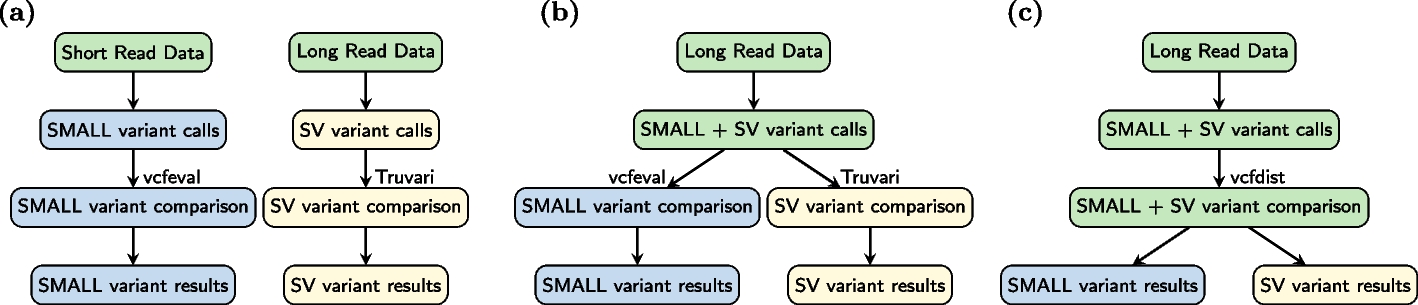
scHolography uses ST and SC data, obtained from tissue-type matched samples, as input (Fig. 1a Input Data). Specifically, scHolography acquires readily available 2D spatial registration from the reference ST data and generates a high-dimensional distance matrix of pairwise pixel-pixel distances from ST spatial registration. Principal component analysis (PCA) is then performed on the distance matrix to select top-ranked PCs and their corresponding values for downstream inferences. We name these top-ranked PCs of the distance matrix as spatial-information components (SICs) (Fig. 1a and Additional file 1: Fig. S1). Interestingly, these SICs capture distinct spatial patterns that are not only observable in the ST reference but also retained in the scHolography reconstruction visualizations (Additional file 1: Fig. S1a-f). To prepare data for model training, ST and SC expression data are then integrated into a shared manifold and SIC values for each ST pixel are defined (Fig. 1a Step1: Data Preparation; see the “Methods” section). Seurat CCA integration is chosen as the default method based on the result from a comparison in our simulated data (Additional file 1: Fig. S2), but different integration methods, such as Harmony, LIGER, and fastMNN, can also be used.

Fig. 1

Overview of the scHolography workflow. a Three steps of the scHolography workflow. (1) scHolography takes in ST and SC expression data and ST 2D spatial registration data. Spatial-information components (SICs) are defined for the spatial registration data. ST and SC expression data are integrated. (2) Neural networks are trained with post-integration ST data as input and top SIC values as the target. (3) The trained neural networks are applied to post-integration SC data to predict top SIC values for SC. SIC values are referenced to infer cell–cell affinity and construct the stable matching neighbor (SMN) graph. The graph is visualized in 3D. b scHolography allows spatial neighborhood analysis. Cells are clustered according to their neighbor cell expression profile. c Based on inferred spatial distances among cells on the SMN graph, scHolography determines spatial dynamics of gene expression. The spatial gradient is defined as gene expression changes along the SMN distances from one cell population of interest to another

Next, scHolography trains neural networks to perform the T2S projection. scHolography utilizes post-integration ST expression data as training input and SIC values as training targets for generating the T2S projection model (Fig. 1a Step2: NN training). The trained model is then applied to SC data to infer spatial cell–cell affinity. The inferred spatial cell–cell affinity matrix is defined as the mean of cell–cell distance between predicted SIC values of runs. The closer distance is correlated with the higher spatial affinity. Finally, the Gale-Shapley algorithm is implemented to find Stable-Matching Neighbors (SMNs) for each cell by using the cell–cell affinity matrix as the matching utility. Cells are matched preferentially with those exhibiting higher spatial affinities through the application of the Gale-Shapley algorithm, chosen for its ability to yield stable matching pairs. This approach ensures that no cell pair would opt for an alternative match over the one currently assigned. The algorithm operates efficiently, employing a sequence of proposals and responses based on ranked preferences, leading to its polynomial time complexity O(n2), where n represents the total number of cells involved. Thus, scHolography uses the collective cell–cell affinity rather than a standalone coordinate to determine the spatial position of a single cell and ensure that every cell is assigned to a unique position, which is constrained by its SMNs. scHolography then visualizes 3D tissue organization by defining the cell–cell spatial connection with an undirected SMN graph and visualizing the SMN graph in 3D by the forced-directed Fruchterman-Reingold layout algorithm (Fig. 1a Step3: Stable Matching Neighbor Assignment).

In the reconstructed tissue, each cell is characterized by its unique spatial neighborhood, defined through the shortest path connecting individual cells on the SMN graph. Tissue spatial heterogeneity can be quantitatively studied not only through the examination of cell types within neighborhoods but also by clustering based on the collective expression profile of cells’ SMNs (see Fig. 1b). Furthermore, both local and global insights into tissue organization can be quantified by ordering cells according to their graph distances from a reference cell type and visualizing gene expression dynamics across the tissue’s spatial continuum (see Fig. 1c). Collectively, scHolography offers a comprehensive solution for 3D visualization of single-cell tissue structures, facilitating the identification of dynamic gene expression patterns and determining spatial cell heterogeneity.

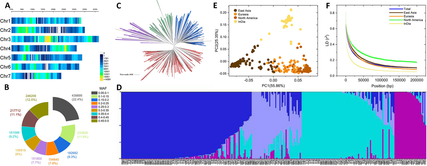
Benchmarking and validation of scHolography

The workflow of scHolography relies on the assumptions that the 2D ST reference dataset contains generalizable information for 3D tissue organization and that cell–cell affinity-based tissue reconstruction provides new insights into tissue organization. To validate scHolography, we first focused on the mouse hippocampus that contains spatially separated regions (Fig. 2a) and used two datasets: a simulated single-cell whole-transcriptome dataset of the mouse hippocampus region with spatial registration information obtained from the Vizgen platform (Vizgen MERFISH Mouse Brain Receptor Map; see the “Methods” section) and scRNA-seq data of the mouse hippocampus [24]. We applied scHolography to both datasets to reconstruct their spatial neighborhoods and visualize the inferred structure in 3D from a 10X Visium mouse brain ST reference data (10X Visium Mouse Brain Coronal Sect. 1 FFPE data). It is worth mentioning that the reference ST slice covers a larger brain region rather than restricted to the hippocampus region whereas the scRNA-seq data were obtained from hippocampus cell populations. We compared the results of scHolography with those from spatial cell charting methods, including Celltrek, CytoSPACE, Seurat, and Tangram. The benchmarking of the methods is based on comparisons using two key metrics: (1) K-L divergence, measuring the discrepancy between the predicted spatial distribution patterns of cells and their ground-truth counterparts, and (2) the average cosine similarity, assessing the alignment between the accumulated expression profiles within the predicted spatial neighborhoods and those within the ground-truth neighborhoods. While K-L Divergence measures a global spatial reconstruction quality, the average cosine similarity measures the accuracy of local neighborhood recapitulation (see the “Methods” section). Across both metrics, scHolography outperforms other methods, achieving the lowest K-L divergence and the highest average cosine similarity (Fig. 2b, c, n.s. (not significant): p > 0.05; *p ≤ 0.05; **p ≤ 0.01; ***p ≤ 0.001; ****p ≤ 0.0001, the same convention applies to all figures). Furthermore, in a focused analysis of the intricate Cornu Ammonis (CA) regions within the hippocampus using annotated scRNA-seq data, only scHolography and Seruat accurately delineate the spatial orders among the CA subfields—CA1, CA2, and CA3 (Fig. 2d–e). This precision contrasts with the difficulties faced by Celltrek, CytoSPACE, and Tangram. These methods encounter challenges due to the ST reference data covering a broader brain area than the scRNA-seq data. This discrepancy leads to non-specific spatial assignments and the erroneous classification of single cells, which should be confined to the hippocampus, across the entire reference space (Fig. 2d). These findings illustrate a critical limitation of 2D spatial cell charting techniques, particularly evident in instances of mismatched regions between ST and SC datasets. To examine the influence of mismatched regions on different computational methods, we performed additional benchmarking using a sub-region of the 10X Visium data that more closely aligns with the simulated SC region. While all evaluated methods showed improved performance on this matched subset, scHolography still demonstrated its superior ability to accurately predict global spatial distribution and effectively differentiate between cell types (Additional file 1: Fig. S3). Despite the dependence of scHolography’s predictions on random seed settings, the consistency of results across various seeds (Additional file 1: Fig. S4a) underscores the robustness of scHolography. Moreover, scHolography enhances model reliability by providing training and validation loss curves of each run and implementing early stopping mechanisms to minimize the risk of overfitting (Additional file 1: Fig. S4b).

Fig. 2

Benchmarking with other spatial cell charting methods. a Illustration of hippocampus CA subfields. b KL-divergence of spatial cell charting method predictions for simulated mouse hippocampus data as ground truth. c Heatmap for the mean of cosine similarity between method-predicted spatial neighborhood accumulated expression and simulated mouse hippocampus spatial neighborhood accumulated expression. The size of the neighborhood varies from 3 to 15 cells. d Visualization of scHolography, Celltrek, CytoSPACE, Seurat, and Tangram single-cell spatial charting results of a mouse hippocampus data. e Comparison of scHolography, Celltrek, CytoSPACE, Seurat, and Tangram results for predicted CA1, CA2, and CA3 cell distance to CA3 cells. Cell distances were normalized for each method by the mean distance between CA3 cells and CA3 cells. f KL-divergence of scHolography predictions for simulated mouse hippocampus data using different ST datasets as references. g Heatmap for the mean of cosine similarity between scHolography-predicted spatial neighborhood accumulated expression and simulated mouse hippocampus spatial neighborhood accumulated expression using different ST references. The size of the neighborhood varies from 3 to 15 cells. h Visualization of scHolography results of a mouse hippocampus data using Slide-seqV2, Xenium, and Merfish ST references. i Comparison of scHolography for predicted CA1, CA2, and CA3 cell distance to CA3 cells using Slide-seqV2, Xenium, and Merfish ST references. Cell distances were normalized for each method by the mean distance between CA3 cells and CA3 cells

Because the core function of scHolography is to generate a T2S projection based on ST and SC transcriptomic measurement, it should be readily applicable for any ST platforms that generate high-dimensional transcriptomic data. To verify its applicability, we next applied scHolography to ST data from diverse platforms, including sequencing-based Slide-seqV2, and imaging-based 10X Xenium and MERFISH. Overall, scHolography successfully delineated tissue structures and accurately assigned single cells to their appropriate spatial neighborhoods, effectively distinguishing between the CA1, CA2, and CA3 hippocampal subfields (Fig. 2f–i). Notably, sequencing-based ST datasets from 10X Visium and Slide-seqV2 yielded better results in terms of K-L Divergence and average cosine similarity (Fig. 2f, g). This enhanced performance can likely be attributed to the deeper transcriptome profiling provided by sequencing-based methods than their imaging-based counterparts.

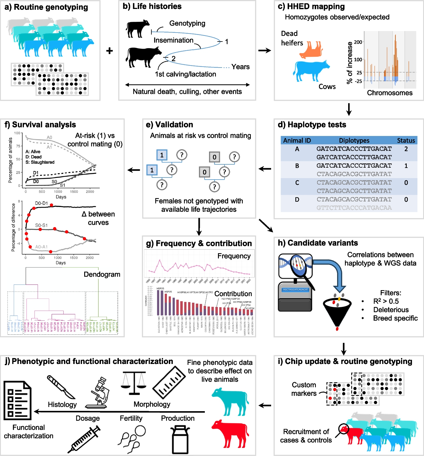
scHolography generates 3D spatial representation from 2D references

To confirm the ability of scHolography to infer 3D tissue architecture from 2D ST references, we used recently published mouse cortex datasets generated by MERFISH, an imaging-based technique, from serial sections [25]. We first selected a single 2D ST slice (slice 400) from the MERFISH dataset for both reference and query in scHolography reconstruction (Fig. 3a, b). To quantitatively evaluate scHolography’s performance, we calculated the SMN distances from various cortical pyramidal neuron layers to the layer 6 (L6) neurons. The results agreed with expected biological patterns: L2/3 neurons were furthest from L6, with L4/5 and L5 neurons progressively closer, and L6 neurons the closest (Fig. 3c). This result confirms scHolography’s ability to recapitulate the stereotypical structure of cortical tissue in 2D.

Fig. 3

scHolography effectively reconstructs 3D tissues from 2D reference. a 2D plot of Merfish mouse cortex data (slice 400). b 3D visualization of Merfish slice 400 scHolography reconstruction result (prediction reference: slice 400; 2D query: slice 400). c SMN distances from L2/3 IT, L4/5 IT, L5 IT, L6 IT to L6 IT in slice 400 scHolography prediction. d Stacked-2D plot of Merfish mouse cortex data (slice 310, 400, and 500). e 3D visualization of Merfish slice 310, 400, and 500 combined scHolography reconstruction result (prediction reference: slice 400; 3D query: combined slice 310, 400, and 500). f SMN distances from L2/3 IT, L4/5 IT, L5 IT, L6 IT to L6 IT in slice 310, 400, and 500 combined scHolography prediction. g Comparison of KL-divergence for scHolography 2D and 3D query results both using 2D reference. h 3D plot of Merfish mouse cortex data (slice 310, 400, and 500) colored by the slice. i 3D visualization of Merfish slice 310, 400, and 500 combined scHolography reconstruction result (prediction reference: slice 400; 3D query: combined slice 310, 400, and 500) colored by the slice. j SMN distances from slice 310, 400, and 500 to slice 310 in slice 310, 400, and 500 combined scHolography prediction

We next applied scHolography to a composite dataset created by stacking slices 310, 400, and 500 from the MERFISH series, with slice 400 serving again as the reference (Fig. 3d). Considering these slices as serial sections from the same sample allowed us to treat the combined dataset as 3D data. The resulting visualizations (Fig. 3e) and layer distance quantifications (Fig. 3f) confirm scHolography’s ability to reconstruct 3D tissue architecture from 2D references, retaining accurate biological structure. Furthermore, comparing the K-L divergence from 2 and 3D queries revealed scHolography’s consistent performance (Fig. 3g). Interestingly, the analysis of distances among cells within each layer underscored scHolography’s precision in capturing subtle spatial differences. The SMN distances for cells in the composite dataset to slice 310 displayed an ascending trend corresponding to the order of slices 310, 400, and 500 (Fig. 3h–j).

To further validate the robustness of scHolography in generating 3D spatial representation from 2D data, we applied scHolography to two MERFISH samples, with Sample 1 comprising six slices and Sample 2 comprising five slices. We used the PASTE algorithm [26] to vertically integrate the slices within each sample, establishing this stacked-2D compilation as the benchmark for ground truth. For each sample, we conducted scHolography reconstruction twice, using either the bottommost or the uppermost slice as the reference point, respectively. Importantly, the fidelity of both reconstructions was consistently high, regardless of the chosen reference slice (Additional file 1: Fig. S5-6). Taken together, these results demonstrate that scHolography can extract cell–cell spatial affinity information from 2D ST references and effectively visualize 3D tissue organization.

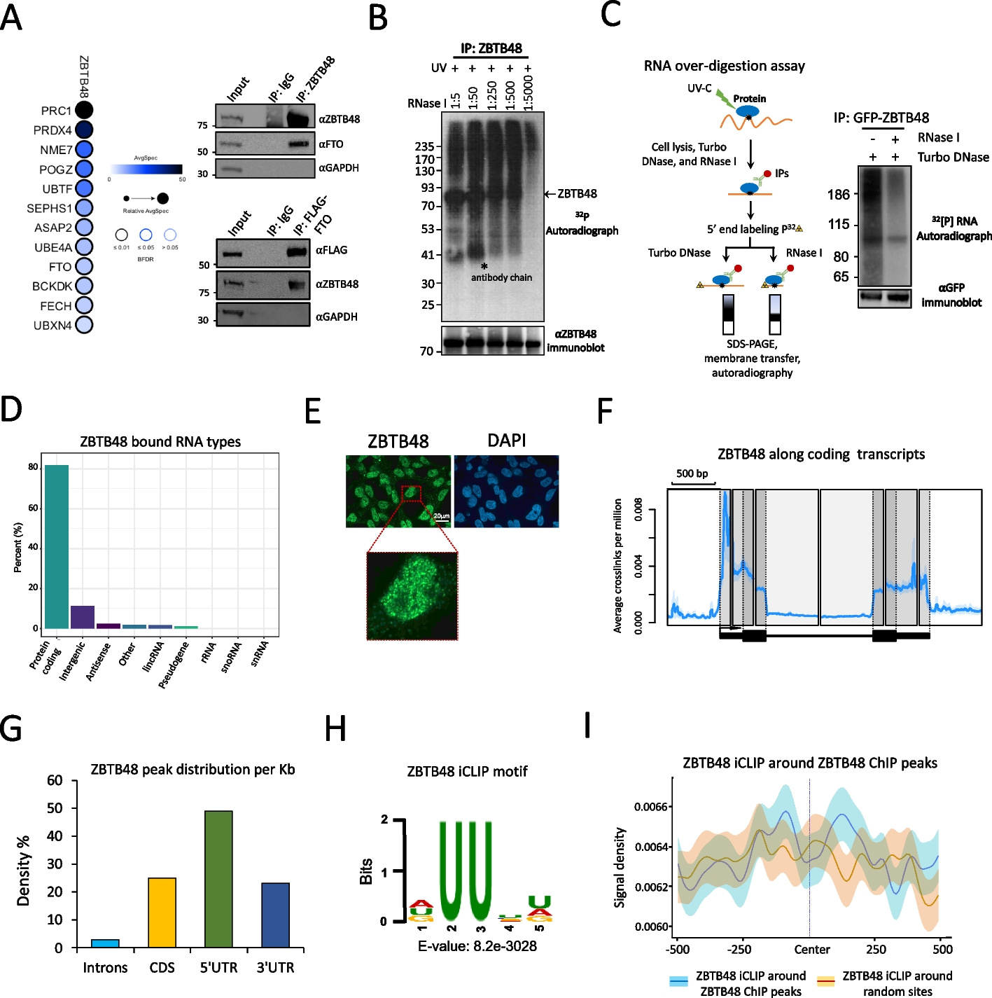
scHolography recapitulates global and local spatial organization of human skin

To test the ability of scHolography to reconstruct tissue organization across different tissue types, we turned to freshly isolated human foreskin samples, whose 3D spatial organization and cell heterogeneity are well appreciated [27, 28]. We generated a 10X Visium ST dataset from a sagittal section of donor #1. This ST dataset captured 659 pixels with a median sequencing depth of 156,332 reads/pixel. By plotting with markers for major skin cell types, we confirmed that our ST data capture all major cell types in the skin, including epithelium, dermal, endothelial and smooth muscle cells (Fig. 4a). We also generated SC data, obtained from a different donor, donor #2, which captured 6425 cells with a mean sequencing depth of 136,235 reads/cell, and 5450 cells passed our filtering with the Seurat package [29]. Unsupervised clustering identified major populations of epithelial and dermal cell types (Fig. 4b). We also detected PECAM1 + endothelial cells, MGST1 + glandular epithelium, CD74 + immune cells, PROX1 + lymphatic endothelial cells, PMEL + melanocytes, MPZ + Schwann cells, and TAGLN + smooth muscle cells (Fig. 4b and Additional file 1: Fig. S7a-b).

Fig.4

scHolography recapitulates the spatial organization of human skin. a Spatial feature plots of markers for four major cell types of human foreskin ST data (KRT10, suprabasal cell; KRT5, basal cell; COL1A2, dermal cell; ACTA2, smooth muscle cell). b UMAP plot of human foreskin scRNA-seq data. c 3D visualization of all cell types in scHolography human foreskin reconstruction. d 3D visualization of four major cell types in scHolography human foreskin reconstruction. e scHolography 3D feature plot of marker genes for 4 major cell. f SMN distances between 4 major foreskin cell types and smooth muscle cells (suprabasal cells n = 1118; basal cells n = 804; dermal cells n = 1529; smooth muscle cells n = 119). Boxplots show the median with interquartile ranges (IQRs) and whiskers extend to 1.5 × IQR from the box. Two-sided Wilcoxon tests are performed. g scHolography 3D plot of Cell #88 and its first-degree neighbors. h SMN cell type composition plot of each human foreskin cell type

We applied scHolography to the SC data to reconstruct the human foreskin at single-cell resolution by using the Visium ST data as the reference (Fig. 4c). scHolography reconstruction recapitulated stereotypical positions of major cell types, reflected by both cell type annotation and gene marker expression in the reconstructed 3D structure (Fig. 4d, e). For example, suprabasal epithelial cells, marked by KRT10hi expression, were located at the outermost layer of the 3D structure, and KRT5hi basal epithelial cells were located beneath the suprabasal cells and sandwiched between the suprabasal epithelial cells and dermal fibroblasts (Fig. 4d, e). The ACTA2hi smooth muscle cells were located at the bottom of the reconstructed 3D tissue, consistent with the stereotypical cell organization of the skin (Fig. 4d, e).

The quantitative measurement of cell–cell distance, inferred by scHolography as the SMN distance, allows the study of tissue architecture based on spatial distance. It enabled us to analyze the distance between individual cell layers. We calculated the SMN distance between suprabasal, basal, dermal, and smooth muscle cells to smooth muscle cells. Not only were the differences highly significant between each cell type (Mann Whitney Wilcoxon test, p < 2.22e − 16), but also the spatial order agreed with stereotypical tissue organization such that suprabasal cells were furthest away from smooth muscle cells, followed by basal cells and fibroblasts (Fig. 2f). Furthermore, because scHolography reconstructed SMN graph designates up to 30 stable-matching neighbors to individual cells as their SMNs (Fig. 4g), we can determine the neighborhood composition for each cell type in the skin by accumulating the SMN cell type information for all cells from each cell type (Fig. 4h). For basal, suprabasal, and glandular epithelial cells, the most abundant neighbors to each cell type were themselves as expected. Notably, fibroblasts often emerged as the most abundant neighbors for cell types that were localized in the dermis, including endothelial cells, lymphatic endothelial cells, and Schwann cells (Fig. 4h). These observations are consistent with the high heterogeneity of dermal fibroblast cells and their complex interactions with other cell types [30, 31]. Together, scHolography reveals spatial cell heterogeneity based on their neighbor cell composition.

Cell type composition analysis identifies transitioning cells during epidermal differentiation

Epidermal differentiation is a dynamic process coupling with spatial cues, where the innermost basal cells, consisting of undifferentiated progenitors, attach to the basement membrane (BM), and differentiating cells delaminate from the BM, remodel their adhesion with neighboring basal cells, and move upward to outer layers as they embark on terminal differentiation to form the protective barrier of the skin [32]. To determine whether scHolography reconstruction recapitulates spatial cell organizations, we investigated the spatial cell neighborhood of epithelial cells defined by scHolography. By plotting the number of basal cell neighbors against the number of suprabasal neighbors for all suprabasal cells, we observed a strong negative correlation among suprabasal cells (R =  − 0.83, p < 2.22e − 16) (Fig. 5a), which indicates that cell composition of the neighborhood could demarcate cellular states of these differentiating cells. Indeed, we readily separated suprabasal cells into two populations: (1) a transitioning keratinocyte population (transition KC) that is defined as suprabasal cells having more basal cell neighbors (more than 1.5 × IQR above the third quartile of the number of basal neighbors of all suprabasal cells) and (2) a terminally differentiated keratinocyte population (differentiated KC) that is defined as suprabasal cells having more suprabasal neighbors (Fig. 5b). 3D visualization of suprabasal and basal cells demonstrated a spatial mixing between transition KC and basal cell populations, whereas the terminally differentiated KC forms a more uniform, outermost layer of the skin (Fig. 5c). Gene expression analysis provided a quantitative view of the transitioning process from basal cells to transition KC to differentiated KC with stepwise decreased progenitor markers (Additional file 2: Table S1-4), including KRT5, KRT14, and COL17A1, and increased differentiation markers, including KRT1, KRT10, and KRTDAP (Fig. 5d). Notably, the downregulation of BM associated genes, such as COL17A1 and COL7A1, is more precipitous than intermediate filament, such as KRT5 and KRT14. Pairwise differentially expressed gene analysis demonstrated that although the transition KC population has higher differentiation marker expression of KRT1 and KRTDAP than basal cells, the differentiated KC population has much higher KRT1, KRT10, and KRTDAP than transition KC, along with additional well-studied terminal differentiation markers LOR, KRT2, and DSC1 [33] (Fig. 5e). In addition, Reactome pathway enrichment analysis [34] identified Keratinization pathway commonly enriched for both transition KC and differentiated KC, whereas Metabolism, Formation of Cornified Envelope, Metabolism of Lipids, and Biological Oxidations pathways were uniquely enriched in terminally differentiated KC (Fig. 5f), consistent with drastically increased lipid and cornified envelope production in these barrier layers. Finally, we examined the expression patterns of the components of Notch signaling, which is known to promote epidermal differentiation [35, 36], in reconstructed basal and transition KC cell layers. Indeed, Notch ligands, including JAG2 and DLL1, are highly enriched in basal cells and strongly downregulated in transition KC (Additional file 2: Table S1), whereas NOTCH3 receptor and canonical Notch targets, such as HES2 and HES4, are strongly upregulated in transition KC (Additional file 2: Table S2). The high granularity of gene expression patterns across these epithelial layers highlights the fidelity of scHolography-based reconstruction.

Fig. 5

scHolography defined SMNs reflect cellular transition in skin epidermal differentiation. a The number of suprabasal SMNs and basal SMNs for each suprabasal cell. b The number of basal SMNs of each transition KC or differentiated KC. c 3D visualization of basal cells, transition KCs, and differentiated KCs in scHolography reconstruction. d Violin plots of epithelial progenitor and differentiation markers. Progenitor markers: KRT5, KRT14, COL17A1. Differentiation markers: KRT1, KRT10, KRTDAP. e Expression dot plots of top 10 upregulated and downregulated genes comparing basal cells vs. transition KC (left) or transition KC vs. differentiated KC. f Reactome pathway enrichment analysis on upregulated genes in transition KC compared to basal cells (top) and on upregulated genes in differentiated KC compared to basal cells (bottom). g Relative incoming (top) and outgoing (bottom) signaling strengths of CellChat inferred significant signaling for basal cell, transition KC, and differentiated KC clusters

The higher spatial resolution of basal and suprabasal cells as well as their neighbors allows us to discern distinct cell–cell communication patterns among three epidermal populations by using CellChat analysis [37]. By incorporating spatial neighborhood information of the epidermal cells, we pinpointed that BM-associated signaling events, such as those mediated by Laminin and THBS, are largely confined within the basal cells. Interestingly, differentiation-associated signaling events, such as those mediated by desmosomes [38, 39], are gradually increased from the basal cells to transition KC and peaking in terminally differentiated cells (Fig. 5g). Furthermore, Notch signaling, which is known to promote epidermal differentiation [35, 36], shows binary patterns between basal and terminally differentiated cells (Fig. 5g). These results not only validate scHolography reconstruction of epidermal layers but also demonstrate the utility of scHolography for studying spatial gene expression patterns.

scHolography reveals spatial heterogeneity in the dermis of human skin

With the ability of scHolography to reconstruct tissue organization with single cells, it raises the possibility of investigating spatial cell heterogeneity with spatially integrated transcriptomes. To do so, we accumulated the expression profile of cell neighborhood for each dermal cell and identify dermal cell subtypes by using distinct transcriptome expression and spatial distribution with the findSpatialNeighborhood function (see the “Methods” section). Four distinct dermal spatial neighborhoods (Dermal1–4) were identified (Fig. 6a–c). Notably, these spatially defined dermal cell populations not only show complex but distinct cell-type composition (Fig. 6b) but also have distinct transcriptome (Fig. 6c). Importantly, scHolography identified spatial neighborhoods differed from the Seurat clusters of scRNA-seq alone (Additional file 1: Fig. S3c). Further scRNA-seq expression analysis on dermal cells from different spatial neighborhoods identified Dermal 1 as papillary dermal cells with high APCDD1 and TWIST2 expression, Dermal 2 as reticular dermal cells with high ADH1B and GREM1 expression, Dermal 3 as endothelial and pericyte-interacting dermal cells with high ABCA8 and IGF1 expression, and Dermal 4 as pericytes with high RGS5 and NOTCH3 expression (Fig. 6d), consistent with experimentally identified derma cell populations [30]. Quantification of the virtual SMN distance (Fig. 6e) and marker gene expression patterns (Fig. 6f) across the reconstructed dermis showed a decreasing trend in the distance between Dermal 1–4 and Dermal 4 cells and unique patterns for each marker, respectively, in line with the notion that papillary dermal cells are located at the upper dermis whereas reticular dermal cells are located at the lower dermis [27, 31]. As a comparison, we also conducted the spatial neighborhood analysis on Celltrek, Seurat, CytoSPACE, and Tangram results, using the same query SC data and reference ST data. While these methods have different spatial charting results, spatial neighborhood analysis from all four methods only identified two spatial neighborhoods (Fig. 6g–j). Combined with the accumulated transcriptome of cell neighborhood obtained from each method, Celltrek and Seurat distinguished pericyte from other dermal cells, while CytoSPACE and Tangram only identified lower and upper dermal cells (Additional file 1: Fig. S7d-g). We also explored the ability of SPOTlight [13], a spot-deconvolution-based method, for spatial neighborhood analysis, combing with the BuildNicheAssay approach described by Seurat V5 [40] on the same SC query data and ST reference data. However, this spot-deconvolution approach failed to capture the differences in the dermal regions, specifically the pericyte, papillary, and reticular regions (Additional file 1: Fig. S8). Taken together, these results demonstrate the superior capability of scHolography not only in reconstructing 3D tissue structures but also in delineating spatial cellular heterogeneity.

Fig. 6

scHolography defined spatial neighborhoods reflect the heterogeneity of human skin fibroblast. a Spatial neighborhood analysis for human skin dermal cells. Four distinct neighborhoods Dermal 1–4 are identified based on the clustering of the accumulated expression profile of dermal SMNs. b Cell type composition of Dermal 1–4. c Heatmap of top 10 differentially expressed genes for Dermal 1–4 accumulated SMN expression profile. d Violin plots of Dermal 4 differentially expressed genes in scRNA-seq data for all dermal spatial neighborhoods. e SMN distances between Dermal 1–4 and Dermal 4 cells. f Expression heatmap of spatially dynamic genes of human dermal cells proximal (left) and distal (right) to smooth muscle cells. Dermal cells are ordered, from left to right, in increasing SMN distance to smooth muscle cells. g–j Single-cell spatial charting results of Celltrek, CytoSPACE, Seurat, and Tangram (left of each panel) and dermal cell spatial neighborhoods identified based on Celltrek, CytoSPACE, Seurat, and Tangram results (right of each panel)

scHolography recapitulates mouse kidney spatial organization

To further examine the performance of scHolography for spatial analysis of tissue organization, we next turned to a complex tissue, the kidney. The kidney plays a vital role in filtering waste from the blood and excreting them through urine, featuring a multifaceted structure segmented into distinct zones that each contributes uniquely to urine production. These spatially and functionally distinct zones include the outer layer cortex, the outer medulla, and the inner medulla, moving from the exterior to the interior of the kidney [41]. Using a combination of micro-dissection and scRNA-seq approaches, it has been shown that proximal tubule (PT) and distal convoluted tubule (DCT) cells are predominantly found within the cortex, whereas collecting duct principal cells (CD-PC) and loop of Henle (LOH) cells are primarily found in the inner medulla. Collecting duct intercalated cells (CD-IC) are distributed throughout all three layers [41]. Applying scHolography to a mouse kidney dataset [22] with a 10X Visium reference (Fig.