1 Introduction

Intuition, as an essential cognitive process in human decision-making and problem-solving, has been extensively described and researched across multiple disciplines, including philosophy (Bealer, 1998), psychology (DePaul and Ramsey, 1998), management (Akinci and Sadler-Smith, 2012), and cognitive science (Nichols, 2004). Intuition involves rapid judgment and processing of information, often occurring at a subconscious level. In psychology, intuitive decision-making is viewed as a swift cognitive process playing a key role in handling complex situations. Slovic and Västfjäll (2010) proposed that in hazardous situations, decisions are made through an automatic processing system reliant on emotions and experience, which is mostly irrational and faster than controlled processing systems. According to Daniel Kahneman's dual-system theory (Daniel, 2017), intuitive decision-making is usually associated with the brain's System 1 thinking, characterized by being fast, automatic, and requiring little cognitive resources. In contrast, System 2 thinking is slower, more logical, and conscious. Moreover, the effectiveness of intuition varies in different application scenarios: experienced pilots can make quick and accurate decisions in adverse weather, seasoned police officers can rapidly identify suspects, and skilled table tennis players can accurately anticipate the ball's landing point and direction in a short time (Cokely and Feltz, 2014). It is this rapid and unconscious decision-making process that plays a vital role in enhancing driving safety.

Driving intuition is a typical manifestation of human brain intuition in real-world scenarios and is an important focus for studying the emergence and development of intuition in complex environments (Risen, 2017). Driving, a daily activity fraught with risks of injury, death, and associated costs, demands high levels of cognitive and sensory engagement from drivers (Abay and Mannering, 2016). Although many manage to maintain safety, the complexity and variability of the driving environment continually pose potential risks. In such contexts, human intuition is pivotal, particularly in collision anticipation. It emerges as a complex cognitive process, where drivers often take preventative actions, like quick braking or steering, before fully realizing the risk (Duma et al., 2017). This preconscious warning in driving scenarios, crucial for emergency responses, might be key in reducing traffic accidents. Recent studies, including those by Liang and Lin (2018), have showed that classical drivers' risk and safe classification could very well be done by using physiological and behavioral measures. Concurrently, Zhang and Yan (2023) has leveraged these EEG indicators to develop a neural network model that estimates collision probabilities at unsignalized intersections.

Existing research has confirmed that the human brain can perceive potential risks before the arrival of danger, a phenomenon that underscores the importance of intuition in driving safety. For example, the study by Kveraga highlights the brain's ability to use past experiences to interpret sensory information and predict the future, particularly in visual recognition (Kveraga et al., 2007). Furthermore, research by Shankaran demonstrates that the brain's response to fear is so rapid that it occurs before conscious recognition, a finding confirmed through the study of the amygdala using ultra-high field magnetic resonance imaging techniques (Ravi Shankaran, 2013). Steingroever et al. (2018)'s study highlights intuitive decision-making mechanisms. Comparing healthy individuals and frontal lobe-damaged patients in the Iowa Gambling Task, they find that healthy participants develop an ability to anticipate and avoid card decks previously associated with net losses (Steingroever et al., 2018). Moreover, the Contingent Negative Variation (CNV), an endogenous component associated with cognition discovered by Walter in 1964, has been linked to event anticipation and motor preparation. Analysis of its waveform composition and brain electrical signals related to prediction has provided new insights into this field (Cohen, 1969; Berchicci et al., 2020; Kóbor et al., 2021; Fiorini et al., 2023). These studies reveal that human intuitive responses in decision-making are driven by complex brain mechanisms, especially in high-risk and rapid-response scenarios such as driving. This involves the coordinated work of brain, including sensory information processing (Frolov et al., 2019), memory retrieval (Rugg and Vilberg, 2013), risk assessment (Brandtstädter et al., 2004; Li et al., 2022), and predicting future events (Ramnani and Miall, 2004; Mullally and Maguire, 2014), enabling drivers to react quickly in emergencies.

1.1 EEG-based functional brain network

With its high temporal resolution and the ability to precisely track neural activity, electroencephalography (EEG) has become a powerful tool for exploring the brain's working state. Especially in improving assisted driving systems, EEG has sparked research interest, such as in driving fatigue detection (Mu et al., 2017; Ma et al., 2019), distraction detection (Li et al., 2021; Zuo et al., 2022), and more, providing important foundations for developing driving safety systems. Additionally, with its temporal resolution far surpassing that of functional Magnetic Resonance Imaging (fMRI), EEG plays a key role in neuroscience research on the brain's decision-making process in fast, unconscious states (Mullinger and Bowtell, 2011). Recent neuroscience studies indicate that the brain's executive capabilities stem not just from the independent roles of distinct regions, but also from their interconnectivity and communication (Stallen and Sanfey, 2015; Lu et al., 2019). Likewise, intuition, a key cognitive function, depends significantly on the interconnectedness and cooperation of brain regions (Kuo et al., 2009; Erdeniz and Done, 2019).

Functional brain networks constructed using EEG serve as an invaluable methodology for the investigation of interdependencies among various cerebral regions (van Straaten and Stam, 2013). These networks facilitate the precise identification and analysis of interconnected and active cerebral regions during intuitive driving, thereby yielding pivotal insights into the neural mechanisms underlying this phenomenon. Currently, this approach has seen extensive application in research pertinent to driving. Notably, Wang observed alterations in the optimal topological structure of the Phase Lag Index (PLI) functional network amidst driving fatigue, with a particular emphasis on the connectivity alterations from frontal to parietal or occipital regions (Wang et al., 2021b). In parallel, Perera et al. (2022) investigated EEG-based driver distraction classification, employing diverse brain connectivity estimation methods. In addition to driving, the combined application of functional brain networks and graph theory analysis has been extended to other scientific fields, including the diagnosis and treatment of neurological disorders (Jiao et al., 2023; Zeng et al., 2024), motor imagery (Gu et al., 2020), and emotion recognition (Guo et al., 2024), thereby underscoring their extensive scientific merit and potential for varied applications.

Current research on the neural mechanisms underlying intuition, particularly in driving, remains limited. The majority of extant research primarily focuses on discerning intuitive predictive behaviors by comparing statistical significances in the time-frequency domains of various EEG signals, which is limited to establishing probabilistic disparities at the level of EEG signals and lacks a robust physiological interpretability (Duma et al., 2017; Jia et al., 2023). Moreover, several studies are limited to the correlation between isolated cerebral region and intuition, thereby neglecting the crucial interplay among different cerebral regions (Kuo et al., 2009; Erdeniz and Done, 2019). Notably, intuition is a dynamic cognitive process involving rapid collaboration and reorganization among cerebral regions, and it can be enhanced through specific training (Fellnhofer et al., 2023). However, most related research focuses on brain activity at fixed time period lengths, neglecting the dynamics of cerebral region activities over time and the individual variability and learnability of intuitive capabilities, thereby failing to explore the temporal evolution of brain connectivity. To address these limitations, a novel approach has emerged: the multi-layer dynamic networks (Han et al., 2020; Chang et al., 2022). This analytical method measures the synchrony of EEG signals across different time windows or bands, integrating the advantages of single-layer networks while emphasizing dynamic characteristics in the temporal dimension.

To address extant gaps in the field, this study represents the first systematic integration of driving intuition, collision anticipation, and dynamic networks. Employing a combination of PLI and the innovative JTF-MDBN approach, we investigated the brain region connectivity changes corresponding to perception, prediction, and response in instantaneous vehicle collision scenarios. By analyzing the dynamic characteristics of brain networks during the initial (ITIP) and advanced phase (ITAP) of intuition training, this research reveals the patterns of brain network activity in situations of emergency evasion or impending collision, identifying significant changes in the brain network during emergency responses. These findings offer new perspectives on understanding the dynamics of brain networks during driving and provide a scientific basis for the development of EEG-based collision anticipation systems and Advanced Driver-Assistance Systems (ADAS). The key contributions of this paper are as follows:

1. Provided a detailed examination of the brain network characteristics during the driving intuition process by analyzing dynamic networks, particularly highlighting the dynamic changes in brain networks at moments of emergency evasion and potential collision.

2. Conducted a comparative analysis of the brain network differences between the initial and advanced phases of intuition training, demonstrating that specific training or stimuli can enhance the effectiveness of intuition.

3. Integrated and evaluated a suite of biomarkers, encompassing multi-layer and single-layer network features(both local and global), substantiating the efficacy of driving intuition biomarkers in collision identification through classification testing.

2 Materials and methods 2.1 Public datasets

We utilized a publicly available EEG dataset named the Simulated Car Crash Anticipation EEG Dataset (SCCA EEG Datasets) (Duma et al., 2017), which focuses on danger perception in intuitive driving. This dataset was collected using a simplified driving simulator as a behavioral task, capturing EEG signals of participants during the process of intuitive driving. The dataset includes EEG recordings from 40 participants using a 32-channel EEG device based on the 10–20 international system (electrode channel positions are shown in Supplementary Figure 1). In the original study, each participant was involved in two task states: “Non-Alert State” (NAS) and “Alert State” (AS).

During the NAS task, participants were required to watch a segment of driving simulation to familiarize themselves with the environment and establish a temporal expectation, with explicit notification that no collisions would occur during this phase. The NAS task consisted of 14 trials, each lasting 7 to 10 seconds. In the AS task, the task involved two possible outcomes: “CrashEnd” (AS-CE) and “NoCrash” (AS-NC). Participants were informed about the randomness of the trial endings and were asked to make an effort to predict whether a car crash would occur. The AS task involved 20 trials each time, with durations randomly varying between 25 to 40 seconds. Collisions occurred randomly in 50 % of the trials.

2.2 EEG preprocessing

In this study, we employed standardized preprocessing steps to reduce noise interference and used signals from the pre-event period to correct for EEG responses during the studied events, thereby controlling for pre-existing differences in brain activity unrelated to the experimental conditions. The preprocessing of EEG data was accomplished through custom programming in MATLAB. The first step in preprocessing involved downsampling the data to a sampling rate of 256 Hz. This was followed by a series of filtering operations targeted at three distinct frequency ranges: theta band (4–8 Hz), alpha band (8–13 Hz), and beta band (13–30 Hz) using finite impulse response (FIR) filters to minimize phase distortions. After filtering, the data underwent further cleaning and formatting, which included the removal of outer channels in the EEG recordings. Additionally, the data was segmented into periods ending with specific events, each with a duration of three seconds, to capture brain activity preceding the occurrence of these events.

Independent Component Analysis (ICA) was applied to identify and remove artifacts using the EEGLAB (Delorme and Makeig, 2004), plugins FASTER (Nolan et al., 2010), and ADJUST (Mognon et al., 2011), where FASTER was utilized for initial automatic artifact detection and ADJUST for fine-tuning artifact removal based on statistical thresholds. Post-ICA, channels containing artifacts underwent interpolation to ensure data integrity and consistency, followed by average reference processing to reduce common noise and enhance data quality. Finally, to investigate the two phases of intuition training, ITIP and ITAP, the study defined the first five experimental trials as ITIP and the last five trials as ITAP.

2.3 Construction of EEG network 2.3.1 Network construction and sliding time window

PLI is a phase-based method for analyzing functional connectivity, utilized to assess phase synchronization between signals from two channels (Stam et al., 2007). This PLI metric is particularly apt for exploring functional connectivity in multi-channel EEG data. It mitigates the volume conduction effects often encountered in EEG signal acquisition, thereby more accurately reflecting true connectivity between brain regions.

PLI=〈sign(Δϕrel(t))〉〉=|1NΣn=1Nsign(Δϕrel(tn))    (1)

Where n represents the time points, and Δϕt denotes the relative phase difference between two signals at time t. The instantaneous phase is calculated using the Hilbert transform. The sign of this phase difference, whether positive, negative, or zero, is determined using the signum function, sign. The PLI is the average of the signs of the phase differences across all time points. Consequently, the PLI value ranges from 0 to 1. A value close to 0 indicates a lack of consistent phase lead or lag relationship between the two signals.

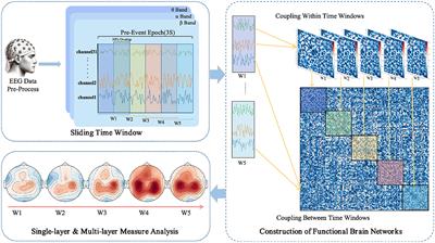
The use of a sliding window method aims to parse the temporal variability in EEG signals, thereby revealing the dynamic integration and reconfiguration processes of the brain's functional networks (O'Neill et al., 2018). As depicted in Figure 1, each task epoch, lasting three seconds, is divided into time windows of one-second width with a step size of 0.5 seconds, resulting in a total of five time windows (W1 to W5). This choice is based on previous research (Chang et al., 2022) and empirical evidence, indicating that these parameters strike a balance between temporal resolution and computational feasibility. For each time window, the PLI values are computed between pairs of EEG channels, yielding a symmetric functional connectivity matrix.

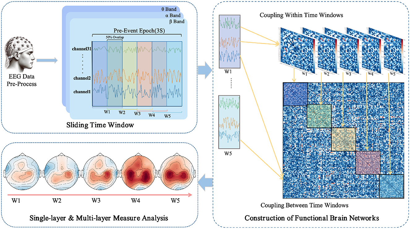
Figure 1. Workflow for EEG data processing and multi-layer dynamic network analysis in anticipation of driving intuition.

2.3.2 Construction of multi-layer networks

Multi-layer networks, integrating multiple single-layer networks, can reveal deeper insights that are not discernible in single-layer networks (Hipp et al., 2012; Boccaletti et al., 2014). In such a structure, each layer shares the same set of nodes, representing different regions of the brain. This configuration encompasses not only the connectivity information among nodes within each network but also includes the connections across different layers. The focus of our analysis will be on the characteristics of the weighted networks both within and between each layer of this multi-layer network structure.

In constructing multi-layer networks, we use PLI to quantify inter- and intra-layer connectivity. For intra-layer connectivity, PLI calculates the likelihood of synchronization between pairs of EEG channels within the time window, thus encompassing the functional connectivity within each different network layer. In contrast, for inter-layer connectivity, PLI evaluates the synchronization between different time windows, thus providing insight into the dynamic interactions between the layers of the network.

To precisely describe the multi-layer network structure in mathematical terms, the concept of a supra-adjacency matrix is introduced (Boccaletti et al., 2014). Specifically, the supra-adjacency matrix can be defined by the following formula:

Asupra=diag(Al)+(H⊗B)    (2)

Where diag(Al) refers to a block diagonal matrix. This block diagonal matrix is composed of the adjacency matrices Al for each layer l within the multi-layer network, where l ranges from 1 to L. On the other hand, (H ⊗ B) represents the connections between layers, where H is a matrix describing the strength and pattern of connections between different layers, B represents a matrix that defines the pattern of inter-layer connections. The symbol ⊗ indicates the Kronecker product. In this study, B is set as E, where E is a matrix composed entirely of ones. Therefore, the matrix constructed in this manner, incorporating both intra-layer and inter-layer connections, can be represented as follows:

Asupra=[A1H12…H1LH21A2…H2L⋮⋮⋱⋮HL1HL2…AL]    (3) 2.3.3 Multi-layer network measures

In the metric analysis of multi-layer networks, this paper primarily employs three characteristic parameters. Firstly, to reveal the coordination consistency between different layers, multi-layer modularity is a concept quantified by the Q-value. The Q-value varies from 0 to 1, representing the degree of network separation from low to high. It signifies the level of separation between different layers (Mucha et al., 2010; Pedersen et al., 2018). The definition of Q-value in a multi-layer context is outlined as follows:

Q(γ,ω)=12μ∑ijlm[(Al−γlkiskjl2ml)δ(Ail,Ajl)+δ(i,j)·ωjml]δ(Ail,Ajm)    (4)

Where γ signifies the cumulative link strength within the multi-layer network. k represents the strength of a node i at the layer l, and m denotes the total degree sum of all nodes at the same layer l. γl denotes the resolution parameters specific to the topology of the layer l, and ωjml symbolizes the inter-temporal connectivity parameter for node j across layers l and m. δ(Ail, Ajm) are 1 for nodes in the same module and 0 otherwise.

To further investigate the brain's integrative and coordinative functions under various conditions, the concept of Multi-layer Participation Coefficient (MPC) is introduced (Boccaletti et al., 2014). It measures the homogeneity of the number of neighbors a node has within a multi-layer network. It is calculated as follows:

MPC=∑i=1NMPCiN=LL-1[1-∑l=1L(ki[l]oi)2]    (5)

where L is the number of layers. MPCi represents the MPCi value of node i within a multi-layer network. MPCi=1 when the degree is the same in all layers and MPCi=0 when a node has non-zero degree in only one layer. ki[l] is the degree in the layer l. oi is the overlapping degree of the node i. The mean MPC for the entire multiplex network is calculated by averaging the individual MPCi values across all nodes.

In addition to the previously mentioned metrics, the multi-layer network can also be evaluated using Layer-Layer Correlation (LLC) Coefficients (Boccaletti et al., 2014). This involves computing the Pearson correlation coefficient between every pair of network layers to assess the degree of correlation among the layers, particularly between layers corresponding to different time windows. The formula for LLC is as follows:

R(Mi,Mj)=∑(Mi−Mi¯)(Mj−Mj¯)∑(Mi−Mi¯)2∑(Mj−Mj¯)2    (6)

Where Mi and Mj represent the matrix blocks from different time windows in the super-adjacency matrix. Mi¯ and Mj¯ are the mean values of the matrix blocks Mi and Mj, respectively.

2.3.4 Single-layer network measures

In the analysis of single-layer networks, we employed two types of classic graph theory metrics. These metrics are crucial for revealing the complex structure and functional characteristics of brain networks (Rubinov and Sporns, 2010). Local metrics delve into the properties of individual nodes or small groups of nodes within the network. Node strength (NS) is defined as the sum of the weights of all edges connected to that node. Path length (PL) is the average distance from one node to all other nodes, reflecting the efficiency of information transfer in the network. Local efficiency (E-loc) reflects the compactness of the “group” of adjacent nodes in the network, and is defined as the harmonic mean of the shortest path between all nodes in the sub-network. Betweenness centrality (BC) is the proportion of all the shortest paths in the network that pass through a given node, with nodes having higher BC values participating in a large number of shortest paths. Eigenvector centrality (EC) takes into account not only the number of connections of a node but also the importance of its neighbors, with higher values indicating that the node is a key player in information transfer and integration. Global indices provide a macroscopic understanding of the performance and characteristics of the network as a whole. The Clustering Coefficient (CC) of a node is defined as the ratio of the number of existing connections among the node's neighbors to the maximum possible number of edges between them. The Assortativity (Ass) coefficient refers to the correlation coefficient between the strengths of the nodes at both ends of an edge, used to measure the correlation between connected pairs of nodes. The calculation methods for single-layer network metrics are shown in Supplementary material.

2.3.5 Statistical methods

Before the main analysis, we verified that our data met the prerequisites for normal distribution and variance homogeneity required by ANOVA. We conducted the Shapiro-Wilk test for normality and Levene's test for equality of variances. Upon confirming that the data met these assumptions, we proceeded with one-way ANOVA to examine differences in multi-layer network metrics, connectivity strengths, and individual single-layer network characteristics across the three task conditions (NAS, AS-CE, and AS-NC). Given the multiple metrics and time windows analyzed, we applied False Discovery Rate (FDR) correction to ensure that the reported effects are robust statistically. Additionally, a single “*” indicates a corrected p-value less than 0.05, “**” denote a p-value less than 0.01, and “***” represent a p-value less than 0.001.

3 Results 3.1 Connectivity of multi-layer networks

Figure 2 illustrates the changes in functional connectivity during intuitive driving, specifically presenting the multi-layer network super-adjacency matrices across theta, alpha, and beta bands in three task states (NAS, AS-CE, and AS-NC) for both ITIP and ITAP. These matrices are derived from the average of all trial data, with diagonal blocks representing coupling within time windows and off-diagonal blocks revealing coupling between time windows.

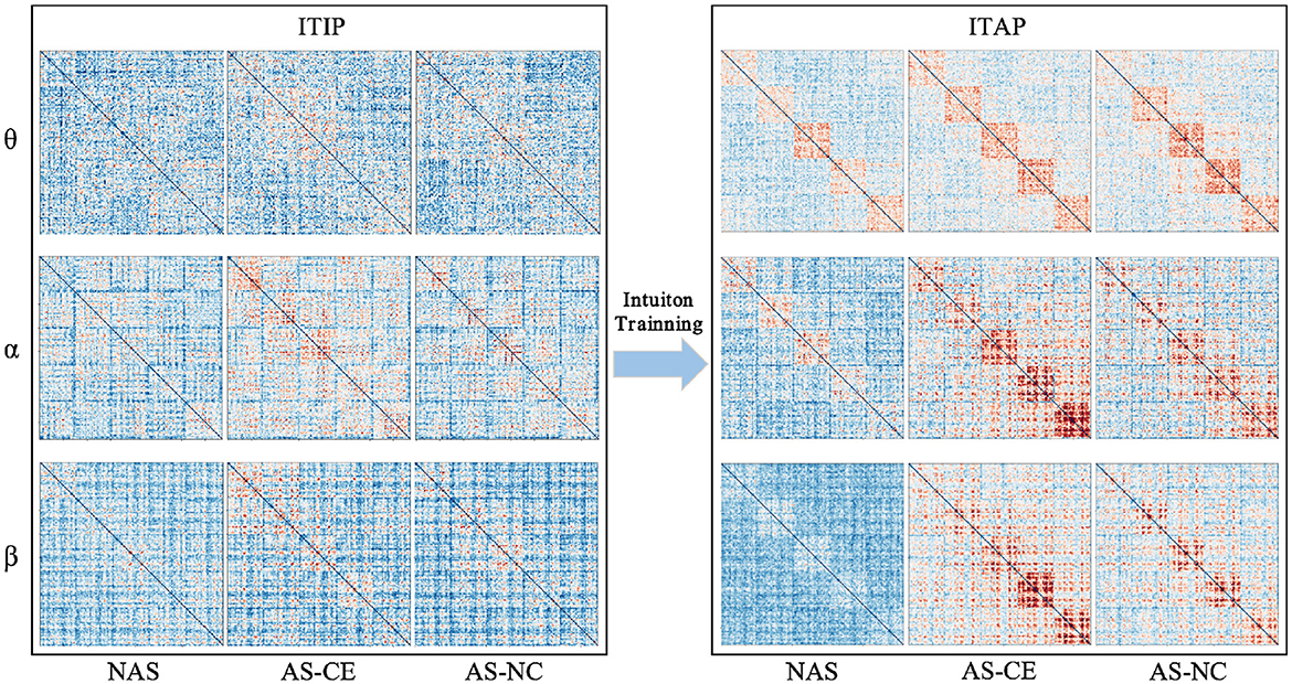
Figure 2. PLI brain network connectivity during initial and advanced phases of intuition training (ITIP vs. ITAP).

The analysis indicates that the PLI connectivity strength within the central diagonal matrix blocks is significantly higher than in the off-diagonal blocks. Notably, during the ITIP, the connectivity patterns observed in the ITAP were absent, suggesting that the brain network during ITIP had not yet formed a stable pattern, rendering it unsuitable for intuition studies. In the ITAP, regardless of theta, alpha, or beta bands, intra-layer connectivity was observed to be markedly stronger than inter-layer connectivity. This was particularly evident in the NAS task, where connectivity levels were significantly lower than in the AS task, including both AS-CE and AS-NC conditions. In AS, enhanced intra- and inter-layer connectivity was observed in time windows W3, W4, and W5. Given these findings, subsequent analyses will primarily focus on the brain networks in the ITAP.

To comprehensively assess the variations in network connection weights during the ITAP under different conditions, we calculated the overall mean of the supra-adjacency matrices for three different experimental conditions (including intra-layer and inter-layer connections), as shown in Figure 3. The results indicate that across all bands, the connection weights for AS-CE and AS-NC are almost identical, while the connection weights for the NAS Task are significantly lower than those for AS-CE and AS-NC. Statistical analyses revealed significant differences between NAS and AS tasks across all three bands. However, the weight difference between AS-CE and AS-NC was not significant (theta: p = 0.5054, alpha: p = 0.3254, beta: p = 0.4367).

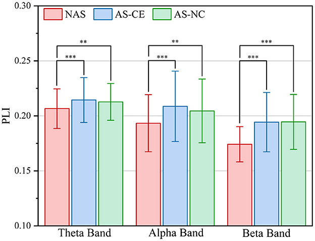
Figure 3. Grand averaged PLI values across task conditions in theta, alpha, and beta bands. **p-value < 0.01, ***p-value < 0.001.

3.2 Graph metrics of multi-layer networks

To highlight those connections that are crucial for functional communication in the brain and to ensure the accuracy and effectiveness of the analysis, this study employed a method based on the statistical distribution of brain network connectivity matrices to determine the threshold for functional brain networks. For each band in Figure 2, we constructed a one-dimensional vector of PLI values for three super-adjacency matrices, which simultaneously consider the values of diagonal and off-diagonal blocks to equally consider connections within and between windows. Then, as illustrated in Figure 4, we analyzed the statistical distribution and Probability Density Function (PDF) of these PLI values. By calculating the 95% confidence boundary, we determined the threshold for the theta band to be 0.2375, for the alpha band to be 0.2349, and for the beta band to be 0.2278.

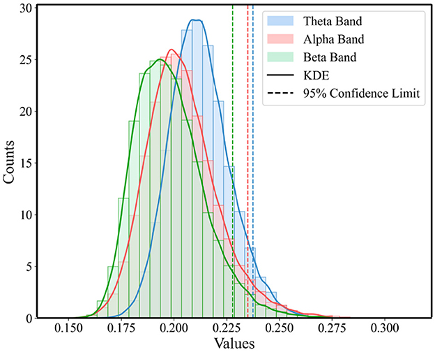
Figure 4. Statistical distribution of PLI value and the PDF for the three conditions across theta, alpha, and beta Bands.

Based on thresholded weighted networks, we calculated three multi-layer network metrics: Q-value, MPC, and LLC. The Q-value results are displayed in Figure 5A using box plots, where the top and bottom boundaries represent the 25th and 75th percentiles, respectively, indicating the distribution of the central 50% of the data. Across all three bands, the Q-value for NAS tasks were found to be higher than those for AS tasks, with significant differences observed in the alpha and beta bands. Additionally, in the theta band, the distribution ranges of Q-value for the three task states were similar, showing no significant differences. A notable distinction was also identified in the alpha band between AS-CE and AS-NC tasks (p < 0.001). However, for MPC, as shown in Figure 5B, the values for the three tasks were similar and did not demonstrate any significant differences.

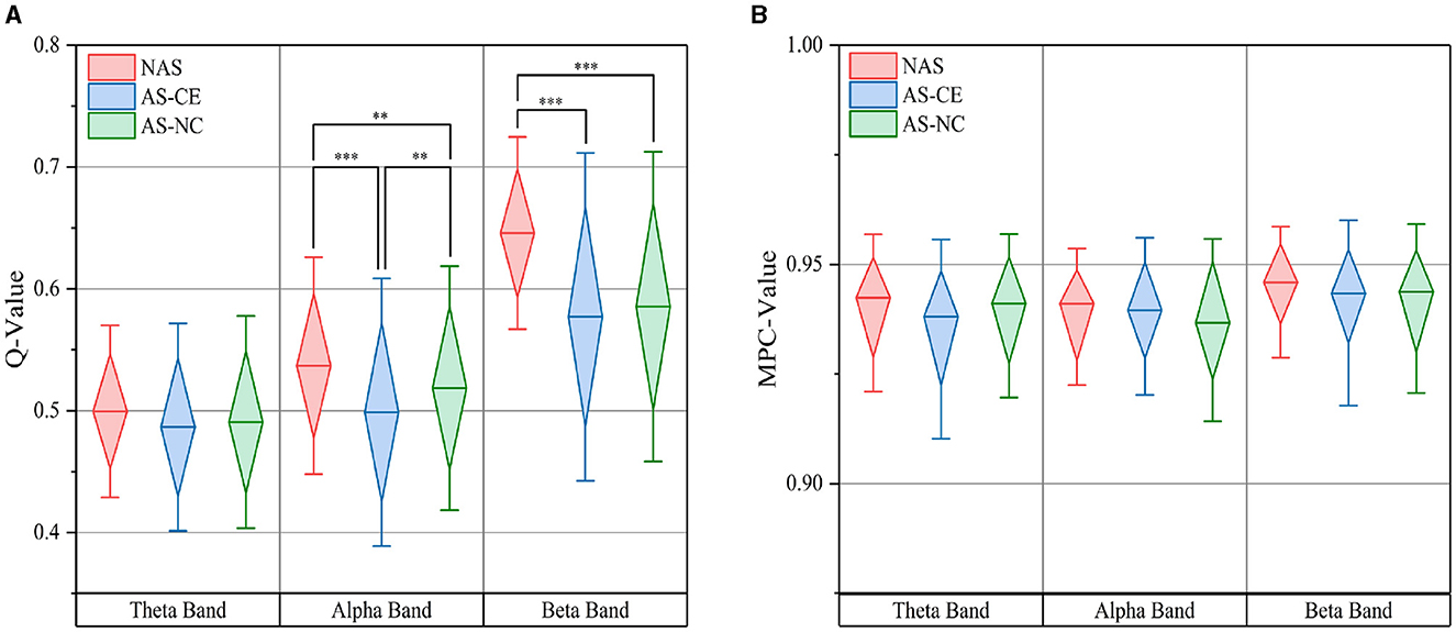
Figure 5. (A) illustrates the distribution of the Q-value, while (B) depicts the MPC value, both measured across theta, alpha, and beta bands under three task conditions. **p-value < 0.01, ***p-value < 0.001.

We calculated the distribution of LLC across different network layers under three task states in the theta, alpha, and beta bands. The observed LLC matrices exhibit symmetry and show higher LLC values between adjacent time windows, which gradually decrease with increasing time intervals. This indicates that the PLI connectivity strength of the brain network maintains a high level of similarity over short time periods, but gradually weakens over longer time scales. After conducting a detailed statistical analysis of the LLC matrices in the theta, alpha, and beta bands, no significant differences were found in the theta band. However, in the alpha band, significant differences in correlations were found between w1 and w5; w2 and w4; as well as between w4 and w5. In the beta band, significant differences were observed between W4 and each of W1 and W3; and between W5 and each of W2, W3, and W4. Figure 6 presents the distribution of LLC across different network layers under three task states in the alpha and beta bands.

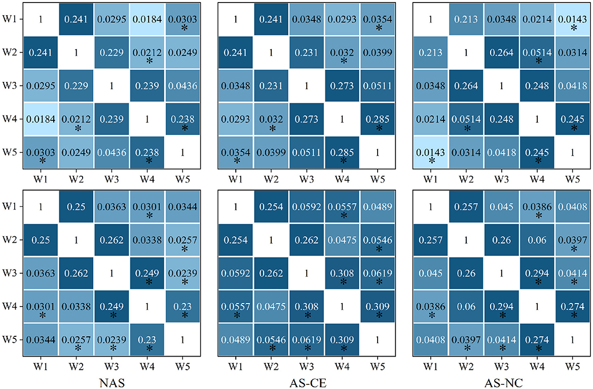
Figure 6. The LLC matrix displays numerical values representing LLC coefficients. “*” mark statistically significant differences between NAS and AS (including AS-CE and AS-NC), The top down is alpha and beta.

3.3 Graph metrics of single-layer networks 3.3.1 Analysis of local metrics

Following an analysis of local graph-theoretical metrics in single-layer networks, significant findings were observed in the NS and E-loc metrics within the Alpha and Beta bands, and did not show any significance in the remaining metrics. Figure 7 illustrates the distribution of these metrics across different task states (NAS, AS-CE, and AS-NC) and time windows (W1 to W5). Figures 7A, B depict the topographical distribution of NS and E-loc in the Alpha band, respectively. It is evident that the NS and E-loc distributions in NAS tasks are significantly lower than in AS tasks. Additionally, significant differences between AS-CE, and AS-NC tasks were observed in some channels during the time window W4 of the alpha band. Similarly, as shown in Figures 7C, D, NAS tasks in the Beta band also exhibited lower values. At time window W5, coinciding with the event occurrence, brain regions showed more intense activities compared to other time windows, with significant differences between AS-CE, and AS-NC tasks in some channels at W5 (Statistically significant channels listed in Table 1. For metrics that did not show statistical significance, please refer to the Supplementary Table S1).

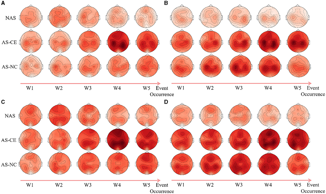
Figure 7. (A, B) Illustrate the topographical distribution of NS and E-loc in the Alpha band, while (C, D) depict the same for the Beta band. Each row corresponds to a distinct task state, while each column represents a specific time window. The intensity of the metric values is depicted through a gradient of color shades.