Introduction

Alterations in mechanical stresses on the glomerular capillaries have been implicated in the progression of glomerulopathy in numerous kidney diseases (Endlich and Endlich, 2012; Kriz and Lemley, 2015; Endlich et al., 2017; Kriz and Lemley, 2017; Srivastava et al., 2017), and the magnitude of the mechanical stresses in the glomerulus depends on the efficiency of autoregulatory control. In the renal microcirculation, the myogenic and tubuloglomerular feedback (TGF) mechanisms of renal autoregulation maintain glomerular blood flow and pressure at optimum levels (Navar et al., 2008). These mechanisms respond to different chemical and physical signals; the myogenic mechanism causes a fast constriction of the afferent arteriole in response to increases in afferent arteriole wall tension, whereas TGF causes slower constriction and is mediated by signals from the macula densa cells that sense increases in tubular fluid osmolality or sodium concentration. Both mechanisms converge at the level of the afferent arteriole smooth muscle cells (SMC), and it is unclear to what degree the TGF and myogenic mechanisms dynamically interact to control SMC tone (Cupples, 2007).

Numerous studies have supported the theory that TGF modulates the sensitivity of the myogenic mechanism (Walker et al., 2000; Walker, 2001; Scully et al., 2013; Mitrou et al., 2015; Scully et al., 2016; Scully et al., 2017); the afferent arteriole constricts faster and with greater magnitude when TGF is intact as opposed to when TGF is inoperant (Walker et al., 2000; Walker, 2001), but it is unclear if this is a result of the TGF mechanism acting additively with the myogenic mechanism, or whether the TGF mechanism directly influences the magnitude and/or kinetics of the myogenic response. Mathematical models of hemodynamic autoregulation allow for the interrogation of hypotheses regarding relative strengths of the myriad factors controlling SMC tone (Carlson and Secomb, 2005; Carlson et al., 2008; Sgouralis and Layton, 2014). We developed a model of renal autoregulation that combines our previously developed model of blood flow and filtration in an anatomically accurate rat glomerular capillary network (Richfield et al., 2020; Richfield et al., 2021) with models of the renal tubule and afferent arteriole to quantitatively characterize interactions between the myogenic and TGF mechanisms and their impact on glomerular mechanics.

The model presented here provides estimates of the mechanical stresses and strains in the glomerular capillaries under different autoregulatory conditions. By modifying the magnitude and kinetics of the autoregulatory mechanisms and their interactions, we estimate each mechanism’s impact on the magnitude of different glomerular mechanical stresses. While previous studies have used mathematical models to comprehensively investigate renal autoregulatory dynamics (Sgouralis and Layton, 2012; Edwards and Layton, 2014; Sgouralis and Layton, 2014; Sgouralis and Layton, 2015; Sgouralis et al., 2016; Ciocanel et al., 2018), no studies have quantitatively related these dynamics to the mechanical consequences experienced by the glomerular cells. Our goal in this study was to quantify the contribution of each autoregulatory mechanism and their interactions to glomerular mechanical homeostasis. Our results indicate that the TGF mechanism directly modulates the sensitivity of the myogenic mechanism, and that this interaction is required to maintain mechanical homeostasis of the glomerular cells when blood pressure is elevated. These findings corroborate previous studies of myogenic mechanism-TGF interaction, suggest mechanisms of glomerular injury in diseases such as hypertension and diabetes, and highlight the utility of mathematical models in probing questions in renal physiology.

Mathematical model

We developed a model of renal autoregulation that portrays the interaction of the TGF and myogenic mechanisms in maintaining single nephron glomerular filtration rate (SNGFR). The model was composed of an afferent arteriole model, a glomerulus model and a tubule model run in series such that the output of each model was used as input for the next (Figure 1). The afferent arteriole model was derived from a model of cerebral autoregulation (Carlson et al., 2008) and the model was fit to data from previous studies that used the juxtamedullary nephron preparation to measure changes in afferent arteriole diameter and flow in response to changes in perfusion pressure (Takenaka et al., 1994; Walker et al., 2000). A glomerulus model previously developed by us (Richfield et al., 2020) was used to estimate magnitudes of SNGFR and mechanical stresses in the glomerular capillaries. To model solute exchange on the length of the tubule, we used a model of solute concentration along the relevant tubular segments (proximal tubule and the descending and ascending limbs of the Loop of Henle) to estimate macula densa solute concentration as a function of SNGFR (Layton et al., 1991). We briefly discuss each sub-model and describe the parameterization of the renal autoregulation model.

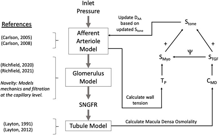
Figure 1. Autoregulation model schematic. Models of the glomerulus and tubule are used to estimate SNGFR and macula densa solute concentration, CMD. The afferent arteriole model calculates wall tension TP, and TP and CMD are used to calculate the myogenic and TGF tones, denoted SMyo and STGF, respectively. The interaction between SMyo and STGF is denoted by Ψ in the diagram and will be referred to as such throughout this article. References are included to indicate the core references used to construct each model, with the novelty of the glomerulus sub-model accentuated.

Glomerulus model

To estimate the effect of alterations in afferent arteriole diameter on glomerular filtration and mechanics, we used a previously developed model of glomerular hemodynamics that models blood flow and filtration throughout an anatomically accurate glomerular capillary network (Richfield et al., 2020). We briefly describe the main equations of the model and discuss our methods for allowing for elastic deformation of the simulated glomerular capillaries, which we have modeled previously (Richfield et al., 2021). Incorporation of an anatomically accurate model of the glomerulus into our model of renal autoregulation constitutes a novel step forward in modeling renal autoregulation, as this model allows us to estimate filtration dynamics and mechanical stress at the glomerular capillary level. This has never been done in previous models of autoregulation.

The anatomical data used in this model were obtained via perfusion fixation and ultrathin sectioning in a previous study (Shea, 1979). The glomerular capillary network used in the model is composed of 320 capillary segments with known length and diameter, and 195 nodes at which the capillary segments bifurcate and/or coalesce. The glomerulus model uses conservation laws to calculate changes in plasma protein concentration and hematocrit as the plasma water is filtered along the length of the network. Thus, for a given systemic plasma protein concentration CA and hematocrit Ht, we calculate the concentration of plasma protein, C and erythrocyte volume in each capillary in the network. Erythrocyte volume is distributed at network nodes nonlinearly according to previously developed empirical models of blood phase separation in the microvasculature (Pries et al., 1996) and the hematocrit in each capillary segment nonlinearly affects blood viscosity according to previous experimental findings (Pries et al., 1994). Improving on previous models of blood flow and filtration in an anatomically accurate rat glomerular capillary network (Lambert et al., 1982; Remuzzi et al., 1992), our glomerulus model does not assume a linear pressure profile on the length of each capillary but instead takes the filtration of fluid into account in calculating the pressure profile p(x). For x = 0 to the capillary length, denoted L, and for Rf the resistance of the glomerular capillary wall to filtration, we obtain the second-order differential equation for the pressure profile:

d2pdx2x−a2px=−a2pBS,(1)

Where pBS denotes Bowman’s Space pressure, a2 = R/(Rf L2) for R the capillary resistance, which we calculate assuming Poiseuille flow. Glomerular model parameters are available in Table 3. The apparent viscosity μ in each capillary segment is nonlinearly dependent on plasma viscosity μpl, hematocrit Ht and the capillary diameter D (Pries et al., 1994):

In contrast to our previous publications (Richfield et al., 2020; Richfield et al., 2021), λ is defined as in (Remuzzi et al., 1992). We obtain the filtered volume or “capillary segment glomerular filtration rate” (CSGFR) by integrating over the length of each glomerular capillary:

CSGFR=∫0Lpx−pBSdxRfL,(3)

and total SNGFR is taken to be the sum of the individual CSGFRs. The filtration resistance Rf is not fixed but is calculated iteratively as a function of plasma protein concentration and the pressure profile on the length of the capillary. According to the fundamental equations of glomerular filtration (Deen et al., 1972) the blood flow through each capillary changes as a function of the pressure profile p(x) on the length of the capillary and the colloid osmotic pressure Π(x) that opposes filtration according to the concentration of plasma protein within the capillary lumen:

dQdx=−kπDpx−pBS−Πx,(4)

For k the hydraulic conductivity of the glomerular capillary wall, defined as the permeability of the wall to water, D the capillary diameter, and

Πx=2.1Cx+0.16C2x+0.009C3x.(5)

(Papenfuss and Gross, 1978). Assuming Poiseuille flow,

Taking the derivative with respect to x,

dQdxx=−LRd2pdx2x=a2px−pBS.(7)

To enforce equality between Equations 4 and 7 we let

Rf=∫0Lpx−pBSdxkπDL∫0Lpx−pBS−Πxdx.(8)

This formulation allows for Rf to be iteratively updated for each capillary segment, as discussed in our previous work (Richfield et al., 2020).

To assess pressure boundary conditions for Equation (10), we calculate the pressure at each network node assuming conservation of blood flow, Q. Specifically, if we let J be the set of nodes j connected to node i, conservation of blood flow at node i is represented by

Where Qij denotes the blood flow between nodes i and j through capillary ij. This relation defines a system of linear equations that can be used to calculate node pressures simultaneously, given pressure boundary conditions at the inlet and outlet, denoted Pa and Pe, respectively. In model simulations, Pa and Pe are set equal to mean arterial pressure and peritubular capillary pressure, respectively.

In addition to predicting aspects of glomerular function, our glomerulus model estimates mechanical stresses in the individual glomerular capillaries. We calculate shear stress, τ assuming Poiseuille flow:

τ=32μ1L∫0LQxdxπD3.(10)

Hoop stresses on each capillary segment, denoted by σ are calculated using the Young–Laplace equation:

σ=D1L∫0Lpx−pBSdx2tGFB,(11)

For tGFB the thickness of the glomerular filtration barrier. Further details of the glomerulus model algorithm and derivation are available in our previous work (Richfield et al., 2020).

In previous iterations of the model (Richfield et al., 2020), the afferent and efferent arterioles were represented as fixed resistors that were tuned to recapitulate rat glomerular hemodynamics in control and disease conditions (Zatz et al., 1986; Kasiske et al., 1988; Franco et al., 2011). In the current study, the afferent arteriole diameter changes as a function of perfusion pressure, which in turn affects pressure and filtration in the glomerulus. In our model formulation the afferent arteriole model determines the change in DAA based on autoregulatory inputs and this diameter is translated to an afferent resistance RAA in the glomerular model. The efferent arteriole length LEA and diameter DEA remain fixed and are used to maintain an adequate glomerular pressure in the control state (Sgouralis and Layton, 2014).

To calculate strain (stretch) of the glomerular capillary walls, we use a constitutive relation assuming that the glomerular filtration barrier is a neo-Hookean solid whereby the hoop stress σ alters the diameter (subscript θ), length (subscript x) and wall thickness (subscript r) of the glomerular capillaries (Richfield et al., 2021):

Where ε denotes the relative change in the glomerular capillary diameter (strain) over the diameter in control conditions, and E is the Young’s modulus of the glomerular capillary walls. Based on data from previous experimental studies wherein glomerular compliance was estimated by quantifying alterations in glomerular volume in response to changes in perfusion pressure (Cortes et al., 1996), we estimate that E for the rat glomerular capillary walls is 14.4 MPa (Richfield et al., 2021). Dividing E by 3 asserts that the wall has the same elasticity in all three directions: axial, radial, and circumferential. In other words, we assume the wall is isotropic, and that the strains are sufficiently small (<10%) to justify a linear stress-strain relationship (Breslavsky et al., 2016). We use this relation to update the diameter, length and thickness of the glomerular capillary walls in response to changes in σ, which allows us to calculate strain of the glomerular capillary walls for a change in arterial pressure. We defer to our previous work (Richfield et al., 2021) for specifics on model implementation.

Afferent arteriole model

The diameter of the afferent arteriole, denoted DAA, changes as a function of the difference between the tension due to blood pressure along the length of the afferent arteriole, denoted TP, and the tension produced by the wall as a function of the myogenic and TGF mechanisms, denoted Twall (Carlson et al., 2008; Sgouralis and Layton, 2014). We use the following differential equation to describe these dynamics:

dDAAdt=1τcTPt−Twallt,(15)

For τc constant (Table 1). The tension of the wall due to blood pressure is modeled as

TPt=Pavgt−PextDAAt2,(16)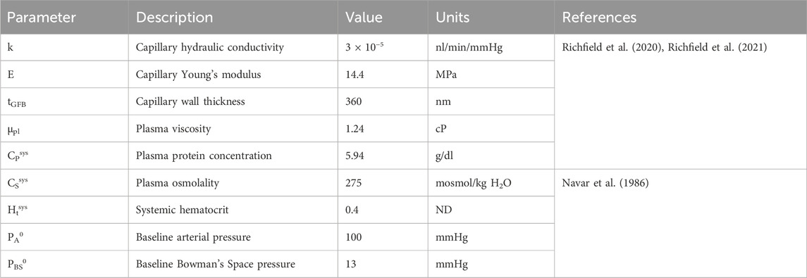

Table 1. Glomerulus model and systemic parameters. ‘ND’ denotes ‘non-dimensional.’

For Pavg the average pressure on the length of the afferent arteriole. The interstitial fluid pressure, Pext, is assumed to be constant and equal to 5 mmHg (Sgouralis and Layton, 2014).

We calculate Pavg given an inlet pressure Pa (equal to arterial pressure) by assuming Poiseuille flow in calculating the total afferent resistance RAA:

RAAt=RRA+128μLAAπDAA4t,(17)

For RRA a fixed resistance provided by the vessels upstream of the afferent arteriole, μ the apparent viscosity of blood as it traverses the arteriole, and LAA the length of the afferent arteriole (Table 2). In previous autoregulation models (Sgouralis and Layton, 2014) the afferent arteriole blood viscosity is increased roughly ten-fold to provide the resistance necessary to maintain control levels of glomerular blood flow and pressure. In our model we take into account the alteration of blood viscosity as a function of vessel diameter and hematocrit (Pries et al., 1994) (described below), thus we model the afferent arteriole segment within a fixed length LAA upstream from the glomerulus and assume a fixed resistance RRA upstream of this main arteriole segment. The baseline diameter DAA0 was selected to enforce a specified baseline glomerular blood flow, pressure and SNGFR, as described below.

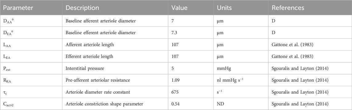
Table 2. Autoregulation model parameters gathered from literature. ‘ND’ denotes ‘non-dimensional.’ ‘D’ denotes ‘derived’ parameter, estimated by fitting the model to data.

The wall tension, Twall is represented by the sum of a passive tension component, Tpass and an active tension component, Tact (Carlson et al., 2008):

The passive tension describes the nonlinear response of the arteriole wall to changes in diameter, independent of the contractile process of the smooth muscle cells (Carlson et al., 2008):

Tpasst=Cpass,1⁡expCpass,2DAAtDAA0−1,(19)

Where DAA0 corresponds to the afferent arteriole diameter at baseline. In general, the superscript 0 indicates the baseline state value, and baseline state values are included in Table 1. The active tension, Tact is a sigmoidal function of smooth muscle cell (SMC) tone, denoted Stone:

Tactt=Cact,11+⁡exp−Stonetexp−DAAtDAA0−1Cact,22,(20)

Where Cact,1 denotes the maximum contractility of the afferent arteriole and Cact,2 is a shape parameter that describes the nonlinear relationship between afferent contractility and the deviation of DAA from the control state (Sgouralis and Layton, 2014). We model Stone as a linear combination of autoregulatory signals:

The myogenic mechanism signal (SMyo) and TGF signal (STGF) are included. We represent each of these signals as functions of their respective inputs: the myogenic mechanism is modeled as a sigmoid function of the change in afferent arteriole wall tension TP from a reference tension TPref and the TGF mechanism is modeled as a sigmoid function of the change in macula densa concentration CMD from a reference macula densa concentration CMDref:

SMyoTP=CMyo,⁡max1+⁡exp −CMyoTP−TPref+CMyo,⁡min(22)STGFCMD=CTGF,⁡max1+⁡exp −CTGFCMD−CMDref+CTGF,⁡min,(23)

Stone = 0 at baseline, thus Stone is not representative of the absolute magnitude of SMC tone, but the deviation of the SMC tone from baseline, wherein a positive Stone elicits a reduction in DAA from baseline and a negative Stone elicits an enhancement of DAA from baseline.

The baseline afferent and efferent arteriole diameters were derived (reference ‘D’ in Table 2) based on the assumption that at the steady-state control arterial pressure, PA0 = 100 mmHg, SNGFR, 30 nL/min, PG, 50 mmHg, and an afferent arteriole plasma flow of 100 nL/min (blood flow QAA, 166 nL/min) (Navar et al., 1986; Richfield et al., 2020; Richfield et al., 2021). We refer to the interaction between SMyo, and STGF, as Ψ, which we discuss in the model parameterization subsection.

Tubule model

To accurately model TGF responses to changes in perfusion pressure, it is necessary to model tubular fluid flow and osmolality up to the macula densa, taking into account the functional heterogeneity along the nephron’s length. In general, we model the change of osmolality CT on the length of the nephron and the tubular fluid velocity v as:

∂CT∂t+v∂CT∂x=−2πrTJs(24)

For v the tubular fluid velocity, rT the tubule radius, Jv the volumetric flux, and Js the solute flux defined as:

Js=JvCTA−PsACT−Ce+VmaxACTCT+Km,(26)

For A the tubule cross-section. Each term in the right-hand side of Equation (26) represents solute transport by a different mechanism. The first term on the right-hand side of Equation (26) represents the reabsorption of solute due to solute drag, wherein water that is transported across the tubule wall carries dissolved electrolytes through the paracellular channel. The volume flux Jv is defined as:

Where the volumetric permeability Pv is a sigmoid function of the velocity:

Pvv=Pv,c1+⁡exp−CTv,1v−CTv,2.(28)

The incorporation of a sigmoid curve into the permeability coefficient Pv is used to assert glomerulotubular balance such that a lack of flow results in a lack of fluid reabsorption. The constants CTv,1 and CTv,2 control the shape of the sigmoid curve. The volume flux is dependent on the difference between the osmolality in the tubule, CT, and the interstitial osmolality, Ce, where

Cex=Ce0=CT00≤x<LPTCe0A1,DL⁡exp−A3,DLx−LPTLDL+A2,DLLPT≤x≤LPT+LDLCeLPT+LDLA1,AL⁡exp−A3,ALx−LPT−LDLLAL+A2,ALLPT+LDL<x≤LPT+LDL+LAL(29)

For L the length of the tubular segment, with subscripts ‘PT,’ ‘DL,’ and ‘AL’ denoting the proximal tubule, descending limb of the Loop of Henle and ascending limb of the Loop of Henle, respectively (Layton et al., 1991). The additional parameters used in these equations are defined as:

A1,DL=1−CeLDLCe01−⁡exp−A3,DL(30)A1,AL=1−CeLALCeLPT+LDL1−⁡exp−A3,AL(33)

The notation Ce (LPT + LDL) refers to a recursive calculation of Ce at x = LPT + LDL, whereas CeLDL and CeLAL refer to the constant expected values of interstitial osmolality at the end of the descending and ascending limbs, respectively (Layton et al., 1991).

The second term on the right-hand side of Equation (26) describes passive solute transport (“leak” of solutes back into the tubule) as a function of the difference in osmolality between the tubule lumen and the interstitium (Ps is the solute permeability parameter). It is assumed that this passive leak only occurs in the ascending limb, where the volumetric permeability is zero and thus passive leakage of solutes is not ameliorated by solute drag as in the proximal tubule and descending limb. The third term on the right-hand side of Equation (26) corresponds to the active reabsorption of solutes, which is a Michaelis-Menten process with maximum uptake rate denoted by Vmax. The Michaelis-Menten constant, Km, is incorporated into this term (Layton et al., 1991).

As stated earlier, each segment of the tubule (assuming three segments: the proximal tubule and the descending and ascending limbs of the Loop of Henle) exhibit different transport processes. This is modeled by altering the parameters depending on the tubular segment (Table 3). Equations 24 and 25 are solved for each segment of the tubule, with the concentration and velocity at the end of the segment acting as the boundary conditions for the next segment (Figure 2). In the steady-state condition, Equations 24 and 25 become:

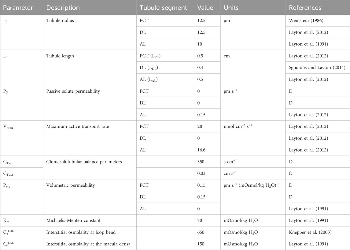
Table 3. Tubule model parameters. ‘D’ denotes ‘derived’ parameter from data.

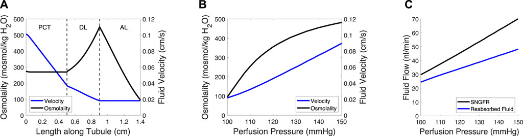
Figure 2. Tubule model predicts osmolality, fluid velocity and the reabsorbed fluid load on the length of the tubule and at varied pressures. (A) Tubular fluid osmolality (black) and velocity (blue) as a function of length along the tubule in the baseline case. (B) Macula densa osmolality (CMD) and fluid velocity at the macula densa as a function of perfusion pressure. (C) SNGFR and the reabsorbed fluid load change with altered perfusion pressure. In (B–C), the afferent arteriole and glomerulus models were used to translate perfusion pressure into SNGFR (Figure 1), assuming no feedback (open-loop). The tubule model was then used to compute macula densa osmolality and fluid velocity (B), as well as the reabsorbed fluid load (C).

The glomerulotubular balance parameters CTv,1 and CTv,2 were estimated to ensure that Equation (35) remained stable at low SNGFR values, wherein the tubular fluid velocity approached 0. We assumed that there was 0 effective passive solute permeability in the proximal tubule (PCT) and distal limb of the Loop of Henle (DL), because the meager impact of passive transcellular transport is dwarfed by the active transport of solutes and solute drag (García et al., 1998). We then adjusted the volumetric permeability Pv,c of the PCT and DL until the fluid flow at the loop bend equaled ∼20% of SNGFR (Layton et al., 1991; Layton et al., 2012) and the CMD = 100 mosmol/kg H2O (Bell and Navar, 1982; Navar et al., 1982), at baseline.

Renal autoregulation model algorithm

The afferent arteriole, glomerulus and tubule models were linked in series, wherein each model fed into the next model, creating a feedback loop (Figure 1). In the model, an input pressure (equal to arterial pressure, assumed 100 mmHg at baseline), is translated into an input pressure and flow for the glomerulus model. The glomerulus model calculates the filtered volume of fluid (SNGFR), which is input for the tubule model. The tubule model calculates the osmolality at the macula densa, denoted CMD. This osmolality and the tension of the afferent arteriole are converted into autoregulatory signals STGF and SMyo, respectively (equations 22 and 23). These are summed and used to modify the afferent arteriole diameter. This feedback loop can be used to simulate transient changes in afferent arteriole diameter, however, we trained our model on steady-state data, as described below. As such, the model was solved assuming that the afferent arteriole diameter is steady-state, and

This assumption implies that the insights we gained from our model are limited to the steady-state stresses exerted on the glomerular capillaries, and the mechanical stresses/strains that these capillaries undergo in transient changes in blood pressure that occur at high speeds. We assumed that we could estimate the latter under steady-state conditions because at the frequency of a rat heartbeat (400 Hz), afferent arterioles are unlikely to change their diameter; studies by Walker et al. showed that, in response to a rapid step in pressure, afferent arterioles take over a minute to fully respond (Walker et al., 2000; Walker, 2001). Any spontaneous oscillations of the afferent arteriole occur at a frequency more than two magnitudes lower than the rat heart rate (Holstein-Rathlou, 1987; Holstein-Rathlou and Marsh, 1990; Holstein-Rathlou and Marsh, 1994; Marsh et al., 2005a; Marsh et al., 2005b). Thus, after parameterizing our model, we used it to evaluate the impact of the autoregulatory mechanisms on transient and steady-state mechanical stresses exerted on the glomerular capillary walls.

Renal autoregulation model parameterization

The mathematical model was partially parameterized using afferent arteriole blood flow data gathered from a previous study (Takenaka et al., 1994). In this study, the juxtamedullary nephron preparation was used to investigate the impact of myogenic and TGF mechanisms on afferent arteriole diameter. A high dose of furosemide was administered to block TGF activity; the same experiment was performed with a papillectomy as the intervention (essentially guaranteeing a loss of TGF), which showed the same results. Additionally, diltiazem, a calcium channel blocker, was used to negate both the TGF and myogenic mechanisms. Using the juxtamedullary nephron preparation, and under each of these experimental conditions, steady-state perfusion pressure was increased from 100 mmHg (baseline) to 150 mmHg, and steady-state afferent arteriole diameter and blood flow were measured.

Our model of renal autoregulation was fit to this data (Figure 3) by using each experimental group as a limit case: the diltiazem data (3 datapoints) were used to estimate the passive parameters Cpass,1 and Cpass,2 (2 parameters) by setting CAct = 0. The maximum active contractility CAct,1 was estimated assuming Stone = 0 in the baseline case and solving Equation (15) assuming steady-state conditions (1 data point, 1 parameter). The Takenaka, 1994 furosemide data (3 data points) were used to estimate the myogenic mechanism parameters CMyo, TPref, CMyo,max and CMyo,min (4 parameters), by setting STGF = 0. To estimate 4 parameters from 3 data points, we assumed that the minimum and maximum SMyo values occurred at pressures of 80 and 180 mmHg, respectively. By assuming that the sigmoid SMyo curve is approximately linear between 80 and 180 mmHg, we estimated CMyo,max and CMyo,min as well as TPref using this assumption, and finally fit CMyo to the original 3 datapoints. Parameterization was performed by minimizing the least squared error between the model QAA and the corresponding Takenaka blood flow data under each of the experimental conditions. To ameliorate issues involving discrepancies between animal and mathematical model baseline state pressure and flow values, the model was fit to the QAA values relative to the model baseline. Importantly, the diltiazem case assumed that the efferent arteriole diameter, as a function of diltiazem concentration, increases at a rate equal to 20% of that of the afferent arteriole as a function of diltiazem dose (Hayashi et al., 2003).

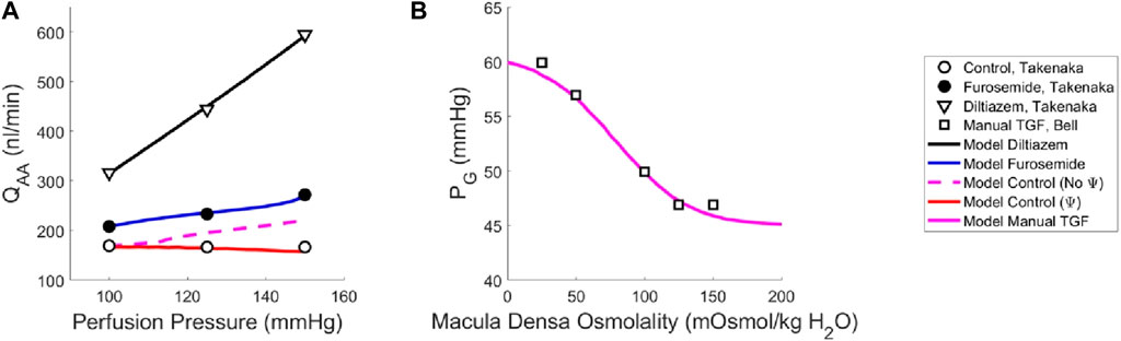
Figure 3. Renal autoregulation model parameterization. Data obtained from literature from Takenaka (Takenaka et al., 1994) and Bell (Bell and Navar, 1982) are represented as points, wherein (A) open circles indicate the control animals, closed circles indicate the animals that received furosemide, open triangles indicate animals that received diltiazem, and (B) open squares indicate animals whose TGF response was manually controlled by placing a wax block in the proximal tubule. Model results are shown as curves, (A) black indicating a passive afferent arteriole, blue indicating only the myogenic mechanism is active, dashed magenta indicates both myogenic and TGF mechanisms are active but do not interact (no Ψ), red indicates that both mechanisms are operant and that the myogenic mechanism sensitivity is modified by the TGF (Ψ). (B) The solid magenta line indicates that the myogenic mechanism is active, but TGF is manually controlled (i.e., tubular fluid concentration is stable, without TGF operant).

To estimate the TGF mechanism parameters, we used data from a different study that measured stop flow pressure changes in response to alterations in tubular osmolality (Bell and Navar, 1982). In this experiment, the myogenic mechanism was operant but the macula densa was cut off from the glomerulus due to a wax block placed in the proximal tubule. As a result, the feedback-isolated TGF response to manual changes in tubular osmolality could be measured in the form of changes in stop flow pressure. Model parameters CTGF, CMDref, CTGF,max and CTGF,min (4 parameters) were fit to this data (5 data points) by estimating the change in afferent arteriole diameter that mediates the changes in glomerular pressure seen experimentally (Figure 3B).

Once we parameterized the steady-state TGF and myogenic signals, STGF and SMyo, respectively, we compared the model output to that of the control condition animals from Takenaka (Takenaka et al., 1994), and showed that the addition of STGF and SMyo (as in Eq. (21)) correctly estimates the control state afferent arteriole diameter at baseline perfusion pressure (Figure 3, dashed magenta). This serves as verification that our model was properly parameterized. However, at higher pressures, the model fails to reproduce the experimental results, as it is unable to constrict to the point where flow is maintained at homeostatic levels. In the juxtamedullary nephron preparation, there is no endocrine signaling to the vasculature and we are not aware of local, paracrine feedback mechanisms that could mediate this constriction other than TGF and the myogenic response. As such, we assumed that the tone required to generate the constrictive response at higher perfusion pressures is generated by the TGF mechanism’s modulation of the myogenic mechanism sensitivity (Walker et al., 2000; Walker, 2001; Cupples, 2007; Scully et al., 2013; Scully et al., 2016; Scully et al., 2017) which we denote Ψ. Namely, we define Ψ as the new set of parameters CMyo and TPref that only are used if TGF is operant:

We recalculated values for CMyo and TPref to create a new myogenic curve (red in Figure 4, entries in Table 4) that fits the control data generated by Takenaka et al. (Takenaka et al., 1994) and calculates Stone as in Equation (21). We fit CMyo and TPref (2 parameters) to the Takenaka control data (3 data points). We included these values in Table 4, distinguishing them from the parameter values associated with the myogenic curve when TGF is inoperant (see Ψ column). By altering these parameters (increasing the slope and shifting the myogenic curve left in Figure 4), the model fits the control data from (Takenaka et al., 1994) and shows adequate control of blood flow QAA (Figure 3). We quantify the model error in supplementary table S1. Because each of the eleven unknown parameters were separately estimated by datasets that contained the same number of datapoints