1 Introduction

With the decreasing cost of high-throughput sequencing data, genomic prediction (GP) emerges as a novel breeding approach, using high-density single nucleotide polymorphisms (SNPs) to capture associations between markers and phenotypes, thereby enabling prediction of genomic estimated breeding values (GEBVs) at an early stage of breeding (Meuwissen et al., 2001). Compared with conventional breeding methods, such as phenotype and marker-assisted selection, GP greatly shortens generation intervals, reduces costs, and enhances the efficiency and accuracy of new variety selection (Heffner et al., 2010).

From the proposal of the concept of genomic prediction to the present, a multitude of models have emerged. Early models primarily focused on improving best linear unbiased prediction (BLUP), such as ridge regression-based best linear unbiased prediction (rrBLUP) (Henderson, 1975) and genomic best linear unbiased prediction (GBLUP) (VanRaden, 2008), etc. In addition, researchers have proposed various Bayesian methods, including BayesA and BayesB (Meuwissen et al., 2001), BayesC (Habier et al., 2011) and BayesLasso (Park and Casella, 2008), Bayesian ridge regression (BayesRR) (da Silva et al., 2021), BSLMM(Zhou et al., 2013). Moreover, bayesian methods generally exhibit higher prediction accuracy than GBLUP in the majority of cases (Rolf et al., 2015). However, the Markov Chain Monte Carlo (MCMC) steps involved in parameter estimation for Bayesian methods can significantly increase computational costs. With advancements in high-throughput sequencing technologies, the increasing dimensionality of genotype data poses new challenges for GP models. To address this problem, some researchers have begun employing regularization term to mitigate the overfitting problem, such as ridge regression (Ogutu et al., 2012), Lasso (Usai et al., 2009), elastic net (Wang et al., 2019). Meanwhile, machine learning (ML) methods such as support vector regression (SVR) (Maenhout et al., 2007; Ogutu et al., 2011), random forest (RF) (Svetnik et al., 2003), gradient boosting decision tree (GBDT), extreme gradient boosting (XGBoost) (Chen and Guestrin, 2016) and light gradient boosting machine (LightGBM) (Ke et al., 2017), have made great performance in genomic prediction methods. With the development of deep learning (DL), researchers have also combined it with genomic prediction models, such as DeepGS proposed by Ma et al. (Ma et al., 2018), based on convolutional neural networks (CNN), and DNNGP proposed by Wang et al. (Kelin et al., 2023) for application in multi-omics, which have achieved better performance compared with other classic models. However, genotype data for most species exhibit high-dimensional small-sample characteristics, leading models often to fail to learn effective features from the training data. Moreover, most GP models contain a large number of parameters and there are significant differences in genotype data among different species, leading to a tedious parameter tuning process for each species, significantly increasing breeding costs. Therefore, enhancing the prediction performance of GP models and reducing the complexity of parameters tuning is of crucial importance for shortening generation intervals and reducing breeding costs.

This study explores a machine learning model, least squares twin support vector regression (LSTSVR), to address above problem. LSTSVR, proposed by Zhong et al. (2012), is a regression model that integrates the ideas of least squares method and twin support vector machine (TSVM) (Jayadeva et al., 2007). LSTSVR contains a kernel function; when linearly inseparable data exists in the original input space, it can become linearly separable after being mapped into a higher-dimensional feature space through an appropriate kernel function (Kung, 2014). LSTSVR improves the computational efficiency during the training process of traditional SVR models by introducing the least squares paradigm to replace the ε-insensitive loss function in SVR, thereby transforming the originally nonlinear optimization problem into an easier-to-solve system of linear equations, offering more stable performance. Simultaneously, adopting a two sets of support vectors for regression enhances the model’s learning capability and robustness (Huang et al., 2013). However, as a general-purpose regression model, LSTSVR still has certain limitations when dealing with various high-dimensional, small-sample genotype datasets.

To better address model overfitting and complex parameter tuning when the number of genotype samples is far less than the number of SNPs markers (Crossa et al., 2017; Tong and Nikoloski, 2020) this study has made improvements and optimizations to LSTSVR. Firstly, inspired by Lasso regularization, a penalty term was introduced to constrain model complexity on LSTSVR. Concurrently, in order to reduce the complexity stemming from model parameter tuning, the subtraction average-based optimizer (SABO) (Trojovský and Dehghani, 2023) was adopted to perform parameter optimization on the LSTSVR model. By combining the Lasso regularization-based ILSTSVR with the efficient optimization of SABO, this study successfully developed a genomic prediction model named SABO-ILSTSVR. To validate the effectiveness of SABO-ILSTSVR, comparative experiments were conducted using SABO-ILSTSVR on four different species datasets (maize, potato, wheat, and brassica napus) against commonly used genomic prediction models (LightGBM, rrBLUP, GBLUP, BSLMM, BayesRR, Lasso, RF, SVR, DNNGP). The results demonstrate that SABO-ILSTSVR exhibits equivalent or superior performance compared with widely-used genomic prediction methods. Finally, in order to reduce the difficulty of using the model, this study provides an easy-to-use python-based tool for breeders to use conveniently.

2 Materials and methods2.1 Dataset

Four different crops datasets are used in this study, including potatoes, wheat, maize, and Brassica napus. The following provides detailed descriptions of the genotype and phenotype data for each dataset.

Potato dataset (Selga et al., 2021) is derived from a total of 256 cultivated varieties across three locations in northern and southern Sweden. Over 2000 SNPs markers used for genome-wide prediction were obtained from germplasm resources at both the Centro Internacional de la Papa (CIP, Lima, Peru) and those in the United States. According to Selga et al. (2021), this number of SNPs is already sufficient for predict genomic estimated breeding values (GEBVs) without loss of information. In this dataset, the total weight of tubers serves as the phenotype data.

Wheat dataset (Crossa et al., 2014) originates from the Global Wheat Program at CIMMYT, comprising information on 599 wheat lines. The project carried out numerous experiments across various environmental settings, with the dataset divided into four core environments according to distinct environmental parameters. Average grain yield (GY) serves as the phenotypic trait data within this dataset. It contains 1,279 SNPs markers, which were acquired following the removal of those with minor allele frequencies below 0.05 and the estimation of missing genotypes utilizing samples from the genotype edge distribution.

Maize dataset (Crossa et al., 2014) originates from CIMMYT’s maize project, comprising 242 maize lines and 46,374 SNP markers. The project encompasses multiple phenotypic data points, and we use the most significant yield-related traits as our phenotype data for this study.

Brassica napus dataset (Kole et al., 2002) is part of the MTGS package. The dataset comprises 50 lines derived from two varieties, 100 SNP markers, and phenotype information on flowering days across three distinct time periods (flower0, flower4, flower8).

2.2 SABO-ILSTSVR model

The SABO-ILSTSVR model integrates the subtraction-based average optimizer (SABO) and an improved LSTSVR method. Its overall framework is depicted in Figure 1, followed by an elaboration of the model.

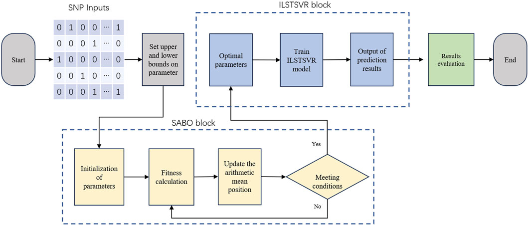
Figure 1. Illustration of SABO-ILSTSVR model frameworks.

2.2.1 LSTSVR

Least squares twin support vector regression (LSTSVR) is an improved twin support vector regression (TSVR) (Peng, 2010; Shao et al., 2013) model by Yang et al. (Lu Zhenxing, 2014). TSVR is an extension of the regression model derived from twin support vector machine (TSVM) (Jayadeva et al., 2007), suitable for addressing continuous value prediction problems, which accomplishes this by determining two regression functions, shown as follows,

f1X=w1TX+b1,f2X=w2TX+b2(1)

where Eq. (1) determines ε-insensitive down-bound function f1 and ε-insensitive up-bound function f2, w1, w2 are weight vectors, b1, b2 are bias term. These can be obtained by solving the following quadratic programming problems (QPPs),

minw1,b1 12Y−eε1−Xw1+eb122+C1eTξ1s.t. Y−Xw1+eb1≥−eε1−ξ1,ξ1≥0,(2)minw2,b2 12Y+eε2−Xw2+eb222+C2eTξ2s.t. −Y+Xw2+eb2≥−eε2−ξ2,ξ2≥0,(3)

where C1, C2 are the positive penalty parameters, ε1, ε2 are up- and down-bound parameters, ξ1,ξ2 are slack vectors, e is a vector of ones with appropriate dimensions. The result of the final regression function is decided by the mean of upper and lower bound functions, as Eq. (4),

fX=12f1X+f2X=12w1T+w2TX+12bl+b2(4)

In the spirit of LSTSVM, Yang et al. apply least squares method to TSVR. TSVR finds the optimal weight vector and bias terms by solving two QPPs, whereas LSTSVR transforms the original TSVR problem into two systems of linear equations for solution, which is typically faster and more stable than directly solving q QPPs, with the loss in accuracy being within an acceptable range. For LSTSVR model, the inequality constraints of (2) and (3) are replaced with equality constraints as follows,

minw1,b1 12Y−eε1−Xw1+eb122+C1ξ1Tξ1s.t. Y−Xw1+eb1=−eε1−ξ1,(5)minw2,b2 12Y+eε2−Xw2+eb222+C2ξ2Tξ2s.t. −Y+Xw2+eb2=−eε2−ξ2,(6)

In formula (5) and (6), the square of L2-norm of slack variable ξ1,ξ2 is used, instead of L1-norm in (2) and (3), which makes constraint ξ1≥0, ξ2≥0 redundant, so the following formulas is obtained,

minw1,b1 12Y−Xw1+eb122+C12 Xw1+eb1−Y−eε122,(7)minw2,b2 12Y−Xw2+eb222+C22 −Xw2+eb2+Y−eε222,(8)

(7) and (8) are two unconstrained QPPs, hence the solutions for w and b can be directly obtained by setting the derivatives to zero, as Eq. (9),

−HTY−ε1e−Hu+c1HTHu−Y−ε1e=0,(9)

where u=wb, H=X e, then, we have Eq. (10) and Eq. (11),

u1=w1b1=1+C12HTH−1HTY+1+C1C1HTH−1HTε1e,(10)u2=w2b2=1+C22HTH−1HTY−1+C2C2HTH−1HTε2e,(11)

thus, the final regression function is fX=12Xw1T+w2T+12bl+b2.

2.2.2 Improved LSTSVR (ILSTSVR)

When applying LSTSVR to handle high-dimensional genotype datasets with small samples, the model is prone to a high risk of overfitting. This is due to the fact that the model may overly fit noise and feature details in the training set, leading to decrease generalization performance on new samples and thereby affecting the effectiveness and reliability of the predictive results. Therefore, this study adds a Lasso regularization term for the weight parameter w in the LSTSVR framework. For linear problems, the function of ILSTSVR is as follows,

minw1,b1 12Y−ε1e−Xw1+b1e22+C12ξ1Tξ1+C32w11+b12s.t. Y−Xw1+b1e=−ε1e−ξ1,(12)minw2,b2 12Y+ε2e−Xw2+b2e22+C22ξ2Tξ2+C42w21+b22s.t. −Y+Xw2+b2e=−ε2e−ξ2,(13)

where C1, C2, C3, C4, ε1, ε2 are positive penalty parameters, ξ1,ξ2 are slack variables, e is a vector of ones of appropriate dimensions. For the non-differentiability with L1 regularization and the convenience of calculations, we assume w1=α*w22, then (12) and (13) can be converted into as follow,

minw1,b1 12Y−ε1e−Xw1+b1e22+C12 Xw1+b1e−Y−ε1e22+C32α1∗w122+b12,(14)minw2,b2 12Y+ε2e−Xw2+b2e22+C22 −Xw2+b2e+Y−ε2e22+C42α2∗w222+b22,(15)

where α1, α2 are vectors of appropriate dimensions, * represents element-wise multiplication. Expand (14) yields,

L=⁡min 12Y−ε1e−Xw1+b1eTY−ε1e−Xw1+b1e+C12Xw1+b1e−Y−ε1eTXw1+b1e−Y−ε1e+C32diagα1w1Tdiagα1w1+C32b12,(16)

let the derivatives of (16) with respect to w1 and b1 respectively be zero, we obtain Eq. (17) and Eq. (18),

∂L∂w1=−XTY−Xw1−b1e−ε1e+C1XTXw1+b1e−ε1e−Y+C3diagα1Tdiagα1w1=0,(17)∂L∂b1=−eTY−Xw1−b1e−ε1e+C1eTXw1+b1e−ε1e−Y+C3b1=0,(18)

composed in matrix form as Eq. (19),

1+C1XTX+C3D11+C1XTe1+C1eTX1+C1eTe+C3w1b1=1+C1XTC1−1XTe1+C1eTC1−1eTeYε1(19)

where D1=diagα1