1 Introduction

COVID-19 disease, due to its rapid spreading worldwide, has led to the most severe pandemic since the deadly Spanish flu, which killed up to 100 million individuals in the past century. Most COVID-19-affected patients have mild symptoms, but approximately 20% of cases need hospitalization, with symptoms characteristic of severe to critical illness requiring very intensive help. Patients with severe illness are often older and/or have comorbidities (e.g., cardiovascular or chronic respiratory disease, diabetes, hypertension, and cancer). Moreover, the organ involvement turned out to be related to disease severity, even though the correlation is still under clarification Daga et al. (2021); Benetti et al. (2020a), while another factor that ended up being discriminant is gender, with men tending to have a more severe disease respect than women Wu et al. (2020). However, these factors do not fully explain the differences in severity and the fact that the immune responses to SARS-CoV-2 were variable, contributing in some cases to greater morbidity and mortality, due to the excessive inflammatory response Ballow and Haga (2021); Madabhavi et al. (2020).

It is now well-recognized that host genetic factors play a fundamental role in the COVID-19 clinical outcome. Recent advances in genome-wide associations have identified potential candidate genes in certain populations that may modify the host immune responses, leading to dysregulated host immunity. Different pathogenetic mechanisms can be involved as new genetic predisposing factors emerge, such as different immunogenicity/cytokine production capability, as well as receptor permissiveness to virus and antiviral defenses. Genetic defects of the type I interferon pathway are linked to a more clinically severe phenotype of COVID-19, and dysregulation of the adaptive immune system may play a role in the severity and complex clinical course of patients with COVID-19 Ballow and Haga (2021). However, with very few genetic factors identified until now, we are still very far from understanding the real relevance of host genetics. The better understanding of host genetic factors is fundamental to predict patients who are at a risk of severe disease and prevent and/or offer personalized and efficient treatments. Moreover, novel genetic discoveries could also inform therapeutic targets for drug repurposing, a pivotal example of which has been the discovery of homozygous deletions in the CCR5 gene conferring resistance to HIV-1 infection, which led to development of a drug that successfully made it through clinical trials Hütter et al. (2013).

Traditional methods for assessing the genetic bases of complex disorders include genome-wide association studies (GWASs) for common variants and burden tests for rare variants. GWASs focus mainly on common variants and are based on a comparison frequency of about 700,000 genomic single-nucleotide polymorphisms (SNPs) in cases/controls (mostly non-coding). The coverage of the coding SNPs is usually performed throughout imputed data, e.g., imputing 2 million SNPs from 700k SNPs by linkage disequilibrium. The method is based on multiple independent tests and has a high threshold for significance. Moreover, GWASs require sample sizes of ten-hundred thousand subjects COVID-19 Host Genetics Initiative (2021); Severe Covid-19 GWAS Group (2020); Kousathanas et al. (2021); Pairo-Castineira et al. (2021). On the other hand, the burden test is based on an aggregation of rare, protein-altering variants and a comparison between cases and controls. The reason behind the burden test is that grouping variants with a large effect size at a gene level might improve power. Like GWASs, the burden test method needs hundreds of thousands of participants for detection of statistically significant associations Kosmicki et al. (2021). These methods have been employed for many years but failed to fully unravel the complexity of human traits. Complex disorders such as COVID-19 are expected to be regulated by thousands of genes with different weights of contribution Marouli et al. (2017); Boyle et al. (2017). Indeed, in common genetic diseases such as cardiovascular or neurodegenerative disorders, the identified genetic markers were not sufficient for full use in clinical practice to predict and treat the disease.

To overcome these limitations, an interplay between host genetics, computational statistics, and dynamic system theory is necessary. Even though the scientific community has made a big effort to analyze the epidemic data made available by the Center for Systems Science and Engineering at Johns Hopkins University Dong et al. (2020), the applications of mean-field models able to predict the kinetics of the epidemic spreading Martelloni and Martelloni (2020a,b); Lai et al. (2020); Chen et al. (2020); Castorina et al. (2020); Fenga (2021); Fanelli and Piazza (2020); Agosto and Giudici (2020); Bialek et al., 2020; Lanteri et al. (2020) cannot help in identifying the gene variants that determine the risk of severity in order to understand the pathophysiological mechanisms responsible for severe disease in heterogeneous groups of patients. At the contrary, machine learning (ML) approaches offer an innovative tool for managing complex problems by significantly increasing our capacity to identify complex patterns of variations. Using data from the whole exome sequencing (WES), a first line of the ML method, i.e., a LASSO logistic regression, has been applied to extract some thousands of coding genetic features contributing to COVID-19 severity Picchiotti et al. (2021); Fallerini et al. (2022). Subsequent functional validation of extracted features demonstrated that, in each tested case, the association with severity has a biological basis and suggested hints for adjuvant treatment Benetti et al. (2020b); Fallerini et al. (2021b,a); Croci et al. (2022); Baldassarri et al. (2021b,a); Mantovani et al. (2022); Monticelli et al. (2021). Using the extracted features, Fallerini et al. (2022) build a severity score named the integrated polygenic score (IPGS), whose performances reached about 75% for both sensitivity and specificity. In this contribution, we want to improve the IPGS severity score performances, with the aim of increasing both metrics and the understanding of biomolecular mechanisms for personalized treatment using innovative ML methods. More in detail, we start from the same set of coding genetic features contributing to COVID-19 severity, already used in Picchiotti et al. (2021); Fallerini et al. (2022), to build two new severity scores that take into account the phenotype of the analyzed patients, i.e., the set of their observable characteristics or traits. In particular, we take into account, in the definition of the severity scores, the involvement of single organs in the development of the COVID-19 disease and the age of patients when they contract the virus. The contribution of single-organ involvement in developing severe COVID-19 disease and that of the gene frequency variants are estimated through an evolutionary algorithm usually implemented to generate high-quality optimization solutions. The severity scores we propose aim at reducing the enormous amount of data to treat and its complexity through a logistic regression, with the final goal of finding a correlation, for each patient, between the score itself and the severity of the disease registered according to the WHO COVID-19 Outcome Scale. In this way, the severity scores cannot be applied as predictive tools in clinical practice since they both require whole-exome sequencing done, the information on organ involvement, and a first screening through a LASSO logistic regression, which is done to extract the coding genetic features contributing to COVID-19 severity. However, they may help in investigating the relationship between gene variants with different frequencies and the development of severe COVID-19 disease.

The Methods section is devoted to the description of the implemented severity scores and the applied methods. Sec. 3 presents the performances of the new severity scores with respect to the IPGS, while a discussion on the presented results is reported in Section 4.

2 Methods2.1 Data collection

Two different cohorts (from Italy and Sweden) contributed to this study, as described in detail in Supplementary Table S1. The Institutional Review Board approval was obtained for each study (see Institutional review board statement below). Information on the cohort demography is given in Table 1.

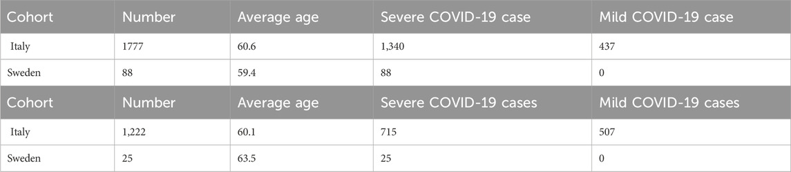
Table 1. Cohort demography information for male (upper table) and female (lower table) patient datasets.

2.1.1 Study participants and recruitment

In order to ensure a collection of samples that could be, as much as possible, comprehensive and representative of the Italian population, hospitals from across Italy, local healthcare units, and departments of preventive medicine have been involved in collecting samples and associated patient-level data for the GEN-COVID Multicenter Study1. The inclusion criteria for the study are as follows: PCR-positive SARS-CoV-2 infection, age ≥18 years, appropriately given informed consent that includes detailed information about the study, and maintaining the confidentiality of personal data. All subjects were positively diagnosed with SARS-CoV-2 and represented a wide range of disease severity, ranging from hospitalized patients with severe COVID-19 disease to asymptomatic individuals. The mean age of patients in the entire cohort is 60.9 years (range 18–99). The patients in the cohort are predominantly men (59.9%) with a mean age of 59.95 years (range 18–99); the mean age of women is 61.8 years (range 19–98). About 30.3% of patients in the cohort have no chronic conditions. The overall case-fatality rate is 2.5% with a mean age of 76.1 years [range 37–98]. Regarding ethnicity, the cohort is composed of 94.25% European, 2.51% Hispanic, 1.09% African, and 2.15% Asian patients. We included all the ethnicities in this study because the results do not depend on population structure-related confounding factors.

2.1.2 Data collection and storage

The socio-demographic information included sex, age, and ethnicity. Information about family history, (pre-existing) chronic conditions, and SARS-CoV-2-related symptoms was collected through a detailed core clinical questionnaire where more than 160 clinical items have been listed (see Supplementary Table S2). Items concerning organ/system involvement (heart, liver, pancreas, kidney, and olfactory/gustatory and lymphoid systems) have been synthesized in a binary mode, where 1 means standard medical parameters indicating specific organ involvement (respiratory severity, taste/smell involvement, heart involvement, liver involvement, pancreas involvement, kidney involvement, lymphoid involvement, blood clotting, cytokine trigger, and a number of comorbidities like asthma, cancer, diabetes, dyslipidemia, hypertension, hypothyroidism, or obesity) and 0 means the absence of involvement of a certain organ/system. Peripheral blood samples were collected in ethylenediaminetetraacetic acid-containing tubes for all subjects, and aliquots of plasma are also available. Whenever possible, leukocytes were isolated from whole blood by density gradient centrifugation and stored in the dimethyl sulfoxide solution and frozen using liquid nitrogen. For the majority of the cohort, swab specimens are also available and stored at the reference hospitals. For more information on data collection and storage, refer to Benetti et al. (2020a); Daga et al. (2021).

2.1.3 Phenotype definitions

COVID-19 severity has been assessed using a modified version of the WHO COVID-19 Outcome Scale (COVID-19 Therapeutic Trial Synopsis 2020); specifically six classification levels have been used to code for the severity: (5) death; (4) hospitalized, receiving invasive mechanical ventilation; (3) hospitalized, receiving continuous positive airway pressure or bilevel positive airway pressure ventilation; (2) hospitalized, receiving low-flow supplemental oxygen; (1) hospitalized, not receiving supplemental oxygen; and 0 not hospitalized. The number of patients present in each phenotype category of this six-level classification (termed GRADING5) is reported in Table 2. Through the application of the presented severity scores, this six-level classification will be reduced to three different classifications: i) a binary classification of patients into mild and severe cases (termed GRADING2), where a patient is considered severe if hospitalized and receiving any form of respiratory support (WHO severity grading equal to 4 or higher in six-point classification); ii) a three-level classification (termed GRADING3), where the patients are classified into non-hospitalized (WHO severity grading equal to 0 or 1), hospitalized and not receiving supplemental oxygen or receiving low-flow oxygen (WHO severity grading equal to 2 or 3), and patients with severe disease (WHO severity grading equal to 4 or higher); iii) a five-level classification (termed GRADING4), where the patients are classified into non-hospitalized (WHO severity grading equal to 0), hospitalized and not receiving supplemental oxygen (WHO severity grading equal to 1) or receiving low-flow oxygen (WHO severity grading equal to 2), hospitalized, receiving continuous positive airway pressure (WHO severity grading equal to 3), hospitalized, receiving invasive mechanical ventilation or dead (WHO severity grading equal to 4, 5).

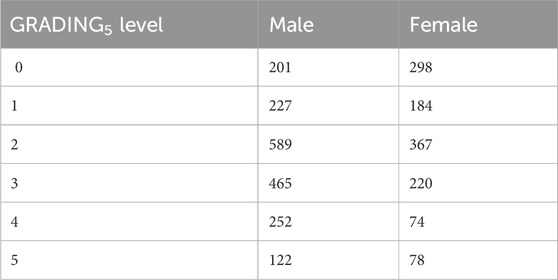
Table 2. Numbers of patients present in each phenotype category for GRADING5.

2.1.4 GEN-COVID cohort

Within the GEN-COVID Multicenter Study, biospecimens from more than 3,000 SARS-CoV-2-positive individuals were collected in the GEN-COVID Biobank (GCB) and used for identifying multi-organ involvement in COVID-19, defining genetic parameters for infection susceptibility within the population and mapping genetically COVID-19 severity and clinical complexity among patients. In particular, within the GEN-COVID Multicenter Study, about 3,000 patients were sequenced by whole-exome sequencing (WES) and partly (about 2,000) already included in the model described in Fallerini et al. (2022). WES with at least 97% coverage at 20x was performed using the Illumina NovaSeq 6000 System (Illumina, San Diego, CA, United States). Library preparation was performed using the Illumina Exome Panel (Illumina) according to the manufacturer’s protocol. Library enrichment was tested by qPCR, and the size distribution and concentration were determined using the Agilent Bioanalyzer 2100 (Agilent Technologies, Santa Clara, CA, United States). The NovaSeq 6000 System (Illumina) was used for DNA sequencing through 150 bp paired-end reads. Variant calling was performed according to the GATK4 (O’Connor and Auwera 2020) best practice guidelines, using BWA (Li and Durbin 2010) for mapping and ANNOVAR (Wang et al., 2010) for annotating.

2.1.5 Swedish cohort

Whole-exome sequencing was performed using the Twist Bioscience exome capture probe and was sequenced on the Illumina NovaSeq 6000 platform. Data were then analyzed using the McGill Genome Center bioinformatics pipeline (https://doi.org/10.1093/gigascience/giz037) in accordance with GATK best practices.

2.2 Post-Mendelian paradigm for COVID-19 modelization

Fallerini et al. (2022) have developed an easily interpretable model that could be used to predict the severity of COVID-19 from host genetic data. Patients were considered severe when hospitalized and receiving any form of respiratory support. The focus on this target variable is motivated by the practical importance of rapidly identifying patients who are more likely to require oxygen support, in an effort to prevent further complications. The complexity of COVID-19 immediately suggests that both common and rare variants are expected to contribute to the likelihood of developing a severe form of the disease. However, the weight of contribution of common and rare variants to the severe phenotype is not expected to be the same. A single rare variant that impairs protein function might cause a severe phenotype by itself after viral infection, while this is not so probable for a common polymorphism, which is likely to have a less marked effect on protein functionality. These observations led to the definition of a score, named integrated polygenic risk score (IPGS), which includes data regarding the variants at different frequencies:

IPGS=nCs−nCm+FLFnLFs−nLFm+FRnRs−nRm+FURnURs−nURm.(1)

In this equation, the n variables indicate the number of input features of the predictive model that promote the severe outcome (superscript s) or protect from a severe outcome (superscript m) and with genetic variants having minor allele frequency (MAF)≥5% (common, subscript C), 1% ≤ MAF<5% (low-frequency, subscript LF), 0.1% ≤ MAF<1% (rare, subscript R), and MAF<0.1% (ultra-rare, subscript UR). The features promoting or preventing severity were identified by an ensemble of logistic models. The weighting factors FLF, FR, and FUR model the different penetrant effects of low-frequency, rare, and ultra-rare variants, compared to common variants (for which the weighting factor has been chosen as 1). Thus, the four terms of Eq. 1 can be interpreted as the contributions of common, low-frequency, rare, and ultra-rare variants to a score that represents the genetic propensity of a patient to develop a severe form of COVID-19. In particular, note the difference in the sign between the severe and mild variants, which, respectively, represent a predisposing factor compared to a protection factor. The model including the IPGS exhibited an overall accuracy of 73% and precision of 78%, with a sensitivity and specificity of 72% and 75%, respectively, thus showing a statistically significant increase in the performances with respect to logistic models that adopt only age and sex as input features. However, in order to design prevention and treatment protocols in view of personalized medicine development, the predictability of the post-Mendelian paradigm for COVID-19 modelization should be further increased.

2.3 First phenotype-based IPGS (IPGSph1)

To improve the ability of the IPGS to predict the severity of the disease, while keeping the linearity of the formula, we first apply vectorial formulation, where both the Boolean variables of the individual patients and the Boolean variables of the single variants are transformed into vectors with components 0 or 1. To each patient and each single variant is associated a vector, which has univocally defined non-zero components: the non-zero components of the patient vector pi and the variants vector vjs,m allow us to codify the situation of each patient who has a unique set of variants and a specific clinical condition when he/she has contracted the COVID-19 disease. Specifically, the clinical overview takes into account the involvement of the organs for each subject that are included in the matrix O, whose entries Oij are 1 (0) in case the organ j is involved (noninvolved) in the disease development of patient i. The organ involvements are grouped into six categories (i.e., heart, liver, pancreas, kidney, olfactory/gustatory, and lymphoid systems), as mentioned in Sec. 2.1. Therefore, the matrix entries Oij take into account, for each patient i, if one of the j = 6 categories are involved (Oij = 1) or not involved (Oij = 0). A scalar product between the vector of the single patient and the vectors of the genetic variants through the matrix of the organs univocally identifies the phenotypic characteristics of the patients, weighted by the variants. Finally, we release the condition that mild variants always protect from a severe outcome, thus being subtracted in Eq. 1, and we do not fix a priori the sign of the mild variants. Starting from a vectorial formulation of the severity score, we are now able to write down a severity score that includes not only the genetic features of the single patients but also the involvement of the organs in the disease development through the matrix of the organs Oij. The score index that encompasses the phenotypical characteristics of the patients is called IPGSph1, and it reads as

IPGSph1=∑fFf∑spiOijvjs+−1α∑mpiOijvjm,(2)

where Ff is the coefficient representing the frequency of the variants, as shown in Eq. 1, and the subscript f identifies either common, low-frequency, rare, and ultra-rare variants. As introduced before, pi represents the single patient vector, while vjs,m represents the vector of severe or mild variants, where we can distinguish between severe and mild according to the superscript. Differently from Eq. 1, we do not fix the sign of the variants; therefore, in the sum over the mild variants, the sign remains a coefficient to be fitted through the parameter α. This results in having 17 more parameters to be fixed. Some examples of Eq. 2 are reported in Sec. 1 in the Supplementary Material; some case examples are specifically reported for different involved organs and different genetic features.

2.4 Second phenotype-based IPGS (IPGSph2)

Inspired by quantum mechanics, we try to generalize the severity score presented in Eq. 2, explicitly introducing in the formula the age of each patient and leaving the possibility, thanks to the quantum mechanics formalism, to introduce into the new severity score expression more general phenotype definitions. For a brief introduction to the quantum mechanics formalism, see Sec. 2 of the Supplementary Material. Borrowing the formalism of quantum mechanics, we use the following elements to construct the second severity score IPGSph2:

• The patient is described in terms of a vector |p >, which represents a state in quantum mechanics and describes the condition of the single human being.

• The genetic variants are also expressed in terms of vectors |vis>, which represent a vector’s basis to calculate the expectation value of the physical observables.

• The organs can be considered the physical observable O, whose expectation value represents our quantum-like IPGSph2.

• The time related to the evolution operator represents the patient’s age.

• The mild or severe variants can be represented through a spin variable s which takes values 1/2 or −1/2.

In order to better clarify the role played by each single element in the severity score, we explicitly write down the values we assign to the new Boolean variables. More in detail, we can distinguish the state of the single i − th patient via assigning a sequence of values pi=10 or pi=01. Since we are dealing with patients who have contracted COVID-19 but have different phenotypic characteristics (i.e., different organs involved in the disease course), the sequence of 2-dim vectors with 0 or 1 values is unique for each patient, and it allows selecting the right organ involvement when performing a scalar product. To gain a better insight into the construction of the severity score, we refer to Sec. 1 in the Supplementary Material. Similarly, the same concept is reported on the genetic variants: if the patient shows the j − th variant, the vector vjs takes the values vjs=10; otherwise, we assign vjs=01. We thus have constructed the quantum-like Boolean variables (or features), and we are ready to define the mathematical structure of IPGSph2:

IPGSph2=∑vis<p|e−ıHtℏOeıHtℏ|vis>,

where H(t) is the Hamiltonian operator and e−ıH(t)ℏ represents the time-evolution operator. To make the previous formula manageable, we perform some approximations, by inserting a completeness of the vectors of our base |vjs><vjs|, which represents the genetic heritage of the human being:

IPGSph2=∑vis∑vjs<p‖vjs><vjs|e−ıHtℏOeıHtℏ|vis>.

We can perform subsequent approximations along two different lines: either i) we suppose that the vectors of the variants are eigenvalues of the Hamiltonian H(t), or ii) we perform the infinite time limit of the system. In the first case, if we assume that Ei represents the eigenvalue of the Hamiltonian H(t) related to the precise state |vis>, we can approximate e−ıEitℏ≃1−Eitℏ. E, corresponding in general to the total energy of the system, can be put in correlation with the comorbidity of the system human being. In this case, we obtain:

IPGSph2=∑vis<p‖vis>∑vjsEj2t2<vjs|O|vis>=IPGS∑vjsEj2t2<vjs|O|vjs>.(3)

In the latter case, the limit t → ∞ corresponds to the assumption that the patient has contracted COVID-19 and his/her status is characterized by a small number of variants that are only those relevant to the contraction/development of the disease. The small set of variants that are related to the disease and influence the clinic outcome of the patients can be called variants of the saddle point Caux (2016) and identified with |vsps>. In this case, the severity score reads as

IPGSph2=∑vis<p‖vis>∑vsps<vsps|O|vsps>=IPGS∑vsps<vsps|O|vsps>.(4)

In both Eqs. 3, 4, the term ∑vis<p‖vis> is present, which represents the scalar product between the vector that identifies the patients’ clinical state and the vector taking into account the genetic variants. Thanks to the characterization of the single genetic variant in terms of the spin variable s (s = mild, severe), this scalar product constitutes the IPGS previously defined in Eq. 1. In other words, the scalar product ∑vis<p‖vis> is the overlap between the initial state, i.e., the state of the patient and the base of our system (the host genetics).

The severity score in Eq. 1 turns out to be corrected by a form factor that constitutes either the expectation value of the organs on the state of all genes, weighted with the age in Eq. 3, or the interplay between the variants of the genes, known to be associated to viral susceptibility and disease severity and patient status in Eq. 4. While the form factor present in Eq. 3 can be easily interpreted as the clinical status of the patient, where organs correlate with the genetic variants, the form factor in Eq. 4 has a more complex interpretation. Somehow, the vector |vsps> represents that the variants selected by LASSO regression in Fallerini et al. (2022) and Eq. 4 can be interpreted as the product between the scores previously defined in Eqs. 1, 2: IPGSph2≃(IPGS)×(IPGSph1).

To summarize, although in the work of Fallerini et al. (2022) the presence or absence of a genetic variant is identified through a Boolean variable 1 or 0, essentially a bit of information, in the present work, in order to maintain the linearity of the problem, we define a quantum bit to identify the presence/absence of a variant. Therefore, we pass from a scalar variable (1 or 0) to a spin variable, thus allowing us to linearly increase the parameter space and improve the prediction of disease severity. Furthermore, being a multifactorial disease, when defining a score in terms of matrix variables, we are able to take age, sex, and organ involvements into account at the same time. In this respect, the mathematics of quantum mechanics seems the ideal environment to describe this type of problem. However, we are just using a quantum-like formalism when replacing Boolean variables with matrices, but we are not introducing any quantum feature in the machine learning algorithm. Irrespective of the fact that we have just taken inspiration from quantum mechanics, since in the previous definitions of IPGSph2, differently from quantum mechanical models, there is no real-time evolution and the vectors are fixed a priori, as well as the structure of the observables, using the quantum mechanics formalism helped us generalize the problem and build a severity score that, in principle, can be generalized to other diseases.

2.5 The genetic algorithm PyGAD

The genetic algorithm is a method for solving both constrained and unconstrained optimization problems that are inspired by natural selection, the process that drives biological evolution. In a genetic algorithm, we start with an initial population of chromosomes, which are possible solutions to a given problem. Those chromosomes consist of an array of genes whose values vary in a predefined range. The whole optimization problem is encoded into a fitness function, which receives a chromosome and returns a number that tells the fitness (or goodness) of the solution. The higher the fitness, the better the solution encoded in the chromosome. The genetic algorithm repeatedly modifies a population of individual solutions. At each step, the genetic algorithm selects individuals from the current population to be parents and uses them to produce the children for the next generation. At each iteration (generation), a number of good chromosomes are selected for breeding (parent selection). Parents are combined two-by-two (crossover) to generate new chromosomes (children). The children are finally mutated by (randomly) modifying part of their genes, allowing for completely new solutions to emerge. Over successive generations, the population “evolves” toward an optimal solution, as it is shown in the flow chart of a genetic algorithm (GA) in Figure 1.

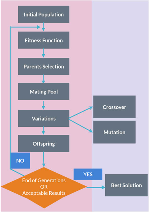
Figure 1. Flow chart of a genetic algorithm.

The genetic algorithm is usually applied to solve problems in which the objective function is discontinuous, non-differentiable, stochastic, or highly non-linear. Among the genetic algorithms, we find PyGAD, an open-source Python library Gad (2021), which supports a wide range of parameters to give the user control over everything in its cycle of operations (see Figure 2).

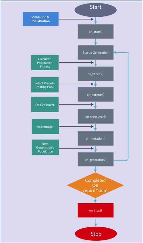
Figure 2. PyGAD lifecycle.

2.5.1 Testing and training procedures

The dataset was randomly divided into a training set and a test set (50/50) for a total of 3,112 patients. In other words, half of the subjects (1,552) were used for training the model, and the remaining half (1,560) are used for testing the model. Patients are chosen randomly to be grouped into the training or the testing set, and the random sampling is varied across the study. Letting the algorithm perform training over a limited set of patients (50%) randomly chosen may potentially diminish the performances of the scores but allows for a more general solution, which is not limited to the particular set chosen for the training/test. The PyGAD algorithm was implemented with the following characteristics in order to converge to a stable solution:

• Number of solutions (i.e., chromosomes) within the population = 32.

• Number of generations 250–500.

• Number of solutions to be selected as parents = 8.

• Parent selection type = sss (for steady-state selection). In the sss case, only a few individuals are replaced at a time, meaning most of the individuals will carry out to the next generation.

• Number of parents to keep in the current population = 1.

• Crossover operation = single_point (for single-point crossover). All genes to the right of that point are swapped between the two parent chromosomes. This results in two offspring, each carrying some genetic information from both parents.

• Type of the mutation operation = random (for random mutation).

• The probability of selecting a gene for applying the mutation operation = 0.2 (for each gene in a solution, a random value with probability 20% is generated).

In most part of the developed training/testing tests, the number of generations able to guarantee a convergence of the solution is 250. We considered a converged solution to be one that has reached an asymptotic value within the duration of the test.

The training/testing procedure, for each severity score, was implemented separately on the male and female patient datasets. The whole procedure is made up of two parts, both used on the testing and training samples. In the first part, we let the genetic algorithm run over the training sample to fit the parameters of the severity scores in Eqs. 2, 3 that produce the best estimate of the N-level classification of patient severity (i.e., GRADINGN parameter). In particular, in this training process, the statistical weights for different organs are calculated without applying any constraint in the fitting process: we do not consider, for example, the possibility that the involvement of certain organs might lead to worse outcomes when compared to that by others. Then, IPGSph1 (IPGSph2) is computed over the test sample by employing the fitted parameters. For each severity score and each dataset, the training and testing tests were repeated 10 times by varying the random sampling. Since the mutation process is random, this is done to ensure that we are able to get the best solution among a sufficient number of iterations. In the second part of the procedure, a multivariable logistic regression is fitted using IPGSph1 (IPGSph2) computed according to the steps described above, together with other input parameters (age, IPGS, and sex), to predict the same GRADINGN parameter. The logistic model is first trained on the training sample and then tested on the test sample. The solutions that are shown in the following section are those corresponding to the best performances among the obtained results.

3 Results

The severity scores in Eqs. 2, 3 are used, together with the GRADINGN data, for training a model that predicts COVID-19 severity. In particular, the training procedure is devoted to fitting the parameters that are present in the severity score equations: 17 free parameters for Eqs. 2 and 18 free parameters for Eq. 3. Fitting the parameters will allow us to assess, for each patient, the level of severity of his/her COVID-19 infection, in terms of IPGSph1 (IPGSph2). Since the final goal is to produce the N-level classification of patient severity, we have to further reduce the results obtainable from Eqs. 2, 3 in the N-level classification along the line of GRADINGN.

To obtain the best possible fit, we have implemented the genetic algorithm PyGAD with the following step fitness function:

• We assign a reward 50 in case the obtained score value is IPGSph1 (IPGSph2) = GRADINGN ± 0.5.

• We assign a reward 5 in case the obtained score value is IPGSph1 (IPGSph2) = GRADINGN ± 1.

• We assign 0 otherwise.

The reward values are chosen without lack of generality: we have assigned a sufficiently big reward value when the algorithm is able to predict the right GRADINGN value, a small but non-zero reward value when the prediction is not too far from the right value and a 0 reward value when the prediction is completely wrong. Any other set of reward values chosen according to this principle, which ensures the convergence of the solution, will give comparable results.

3.1 GRADING2

First, we present the results related to GRADING2, where we have reduced the severity scores to a binary classification of patients into mild and severe cases, considering a patient severe (GRADING2 = 1) if hospitalized and receiving any form of respiratory support or healthy (GRADING2 = 0) in all the other cases. The number of patients present in each phenotype category for GRADING2 is reported in Table 3.

Table 3. Numbers of patients present in each phenotype category for GRADING2.

Furthermore, a multivariable logistic regression was fitted using possible inputs IPGSph1 and IPGSph2, alone or combined with IPGS, age, and sex. Figure 3 shows the confusion matrices, also known as error matrices Stehman (1997), for the male (panels (a) and (b)) and female (panels (c) and (d)) patient dataset, where the best fit is presented for both sets. The performances of the logistic regression increase when multiple predictor variables are used, instead of the single severity score IPGSph1 (IPGSph2). In particular, the best fit is obtained, both for the male and female patient dataset, when using age, IPGS, and IPGSph1 (IPGSph2) as inputs, while for male patients, the new severity score