Dataset

To train and test our prediction model, we used human gut microbiome data, for which both 16S sequencing and WGS platforms were applied to the same sample. Through an extensive search, we identified three published datasets (Winglee et al. 2017; Laudadio et al. 2018; Peterson et al. 2021). A brief description of each cohort is provided in Table 1. Below, we explain how we processed the raw data from these three cohort datasets.

Table 1 Summary of the three cohort datasets used for MicroPredict training and testResonance cohort

In the RESONANCE cohort, there were 648 individuals, including human stool sample data from 348 children and 300 mothers (Peterson et al. 2021). Sequencing of the V4–V5 region of the 16S rRNA gene was performed using SRA (NCBI BioProject PRJNA695570), yielding raw sequencing data (.fastq). For more information about the cohort, please refer to the original manuscript.

Urban and rural Chinese (URC) cohort

In the URC cohort, there were 40 samples of 20 urban and 20 rural people from southern China (Winglee et al. 2017). Sequencing was performed on the V4 hypervariable region of the 16S RNA. Raw sequencing data (.fastq) were obtained using SRA (accession number: SRP114403). For more information about the cohort, please refer to the original manuscript.

Crohn disease (CD) cohort

In the CD cohort, six different stool samples (three healthy controls and three CD samples) were collected (Laudadio et al. 2018). We used these data as additional independent test data to evaluate the prediction methods because they were too small to train the model. Sequencing of the V4–V5 region of the 16S RNA gene was performed using SRA (NCBI BioProject PRJNA349463), yielding raw sequencing data (.fastq). For more information about the cohort, please refer to the original manuscript.

Multi-cohort

The RESONANCE and URC cohorts were combined to create a merged cohort. We referred to this cohort as the “Multi-cohort.” To build the final prediction model for users, this Multi-cohort model was used to maximize the number of samples used for model building.

Taxonomic assignment and quality control (QC)

To profile the microbial communities, we processed the 16S sequencing data using QIIME2 (Quantitative Insights into Microbial Ecology 2 - q2cli version 2021.11.0) with the dada2 plugin (Callahan et al. 2016; Bolyen et al. 2019). We used version 138 of the SILVA database to classify the taxonomy of the reads (Quast et al. 2013). We then filtered low-quality bases and artifacts (barcodes, adapters, and chimeras) and profiled shotgun sequencing data via KneadData v0.10.0 (https://bitbucket.org/biobakery/kneaddata) and MetaPhlAn (version 3.0; 20 Mar 2020 with mpa v30 ChocoPhlAn database) (Beghini et al. 2021). KneadData uses trimmomatic v.0.39 (Alneberg et al. 2014) and Bowtie 2 version 2.4.4 (Langmead and Salzberg 2012) for trimming low-quality reads and aligning sequencing reads to the reference. There are eight hierarchy levels in taxonomic classification; however, we focused only on the lowest taxonomic rank (e.g., species-level) of the taxonomic abundance profiling of metagenomic datasets.

In the RESONANCE cohort, we used all data, including those from adults, to maximize the sample size. As this was a longitudinal study, there were multiple (nine) time points. The earliest time point was selected for each sample. Additionally, we excluded samples that were not paired on either sequencing platform. The data comprised 405 participants: 337 children and 68 mothers (Table 1). We used the child/mother indicator and time point as covariates to control for sampling bias and adjust for significant differences in microbiome composition across conditions. The taxonomic assignment of this cohort resulted in 751 species. A total of 40 samples from the URC cohort were used. Taxonomic assignment resulted in the abundance data for 285 species at the species-level. We used all six samples from the CD cohort. Taxonomic assignment resulted in abundance data for 170 species at the species-level after processing the raw data.

After taxonomic assignment and QC, the taxa were divided into three groups: taxa detected by both platforms, the WGS platform only (WGS only), or the 16S sequencing platform only (16S sequencing only). Table 2 lists the number of species in each group. As expected, WGS was more sensitive for detecting taxa at the species-level compared to the 16S sequencing platform. This contrasts with the results at the genus level, where more taxa were detected by 16S sequencing (Supplementary Table S1).

Table 2 Summary of the number of the species for each platform in the three cohortsData normalization

Data normalization was required because QIIME2 for 16S sequencing yielded absolute abundances, whereas MetaPhlAn3 for WGS provided relative abundances. To match the units of the two methods, we converted the absolute abundances of the 16S sequencing data to the relative abundances using the QIIME2 “feature-table relative-frequency” function.

After transforming all abundances into relative abundances, we normalized the samples by library size (i.e., total counts). After dividing by the total counts, we multiplied by 106 and applied the log10 transformation to the count values. To avoid infinite values, we added 1 to the values before the logarithmic transformation. This normalization helped us apply our linear mixed model because the original data were likely from count distributions (Poisson or negative binomial) rather than from normal distributions (Dobson and Barnett 2018).

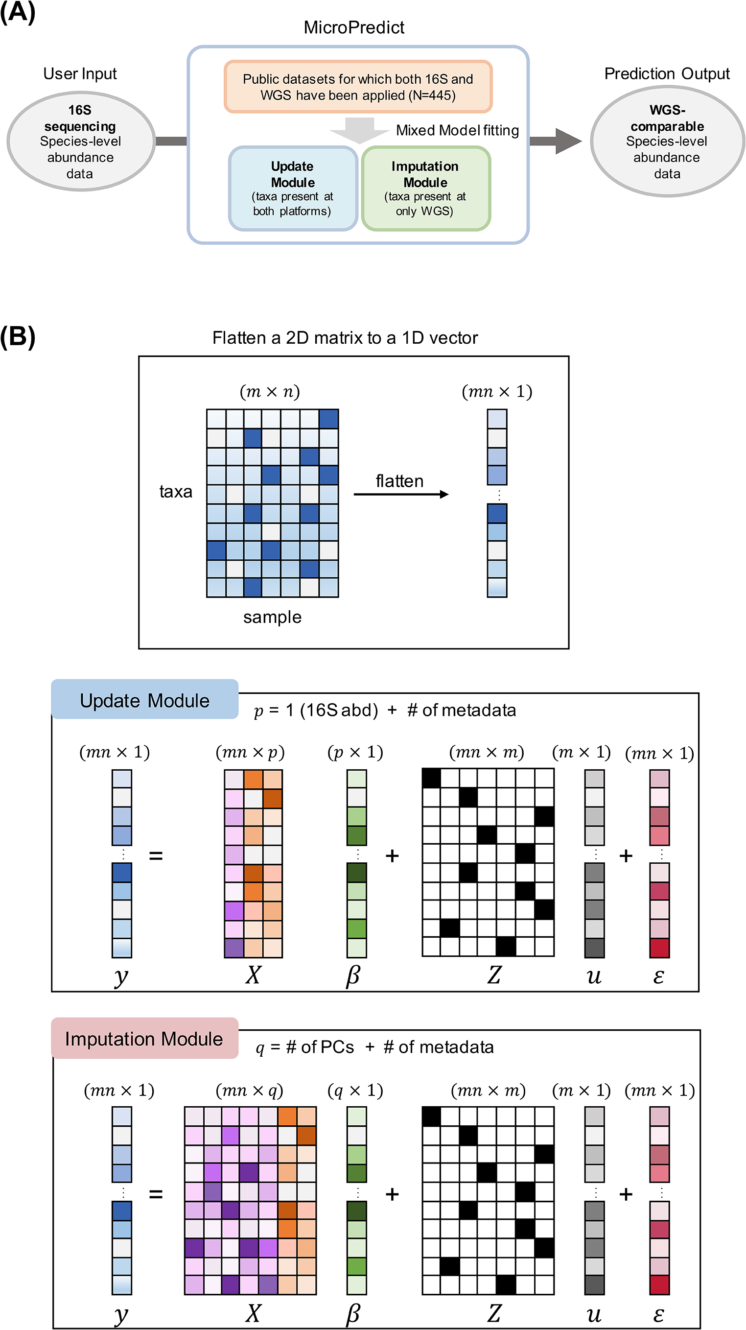
MicroPredict

We developed MicroPredict, a statistical method that predicts the taxonomic profiles of species-level abundance data using 16S sequencing abundance data. Figure 1A presents an overview of the proposed model, MicroPredict. In this model, we assumed that users had only low-cost 16S sequencing data and aimed to predict the species-level abundance data that would be obtainable using WGS technology. Hence, users can provide a count matrix from the 16S sequencing data as input.

MicroPredict consists of two modules: an update module and an imputation module (Fig. 1A). We first applied the update module to remove possible 16S-specific biases for species present in both platforms. We then applied an imputation module to impute species that were absent in 16S but present in WGS.

Update module

The update module was designed to predict the taxa detected by both 16S sequencing and WGS. Although these taxa were detected by both platforms, the estimated abundance of these taxa was usually different. This may be because the total number of detected taxa (common denominator) was different or because each platform had its own bias. Here, we assumed that WGS is the gold standard and chose to update the abundances from 16S sequencing to the values estimated by WGS. To this end, we constructed the following linear mixed model:

$$y\, = \,X\beta \, + \,Zu\, + \, \epsilon \,$$

(1)

\(u \sim MVN(0,\sum ),\varepsilon \sim MVN(0,}),n\) is the number of samples, and m is the number of taxa exclusively observed in the WGS platform. \(y\in ^\) is a vector of WGS abundance, and \(X\in ^\) is a design matrix consisting of \(p\) variables (\(p=3\):16S sequencing abundance data, binary metadata, and time point). The metadata variables for the three cohorts are presented in Table 1.

\(\beta \in ^\) denotes fixed effects. \(Z\in ^\) is a design matrix of \(m\) taxonomic species, and \(u\in ^\) denotes random effects modeling species-specific effects. \(\varepsilon\in ^\) is a vector of the residuals (random errors). We assume that these two random variables \(u\) and \(\epsilon\) follow multivariate normal distributions (MVN), where \(\varSigma\) is a covariance matrix for random effects \(u\). The unknown parameters of this model are \(\beta\), \(\varSigma\), and \(^.\) A schematic of the mathematical structure and dimensions of the proposed model is shown in Fig. 1B.

The rationale behind this mixed model is as follows. The fixed-effect term (\(X\beta\)) accounts for the sample (individual)-specific effect. The 16S rRNA abundance values of each sample for the same taxa were used as fixed-effect predictors. The random-effects term (\(Zu\)) models species-specific effects and cross-species correlations. Specifically, species-specific effects were modeled by equivalent shifts in taxa for the same species across all samples. In addition, microbial taxa share evolutionary information that can be used to generate a phylogenetic tree. For example, taxa that are closer together in a phylogenetic tree are likely to share more common features than those that are further apart. The covariance structure (\(\varSigma\)) encodes these dependencies in the microbiome as correlations between species. We found that prediction accuracy was maximized only when both sample- and species-specific effects were accounted for (as shown in the Results).

Imputation module

The imputation module imputes taxa that are detectable only by WGS using 16S data. We used a linear mixed model similar to that applied in the update module. The only difference was the use of 10 principal components (PCs) as the fixed-effect predictor instead of the 16S sequencing abundance data of the corresponding taxa (Fig. 1B). The linear mixed model for the imputation module is expressed as follows:

$$y = X\beta \, + \,Zu\, + \, \epsilon$$

(2)

where \(u \sim MVN(0,\sum ),\varepsilon \sim MVN(0,})\) and \(X\in ^\) is a design matrix consisting of \(q\) variables \(\left(q=12\right). q\) variables were composed of the top 10 sample-specific PCs calculated from the 16S sequencing taxa abundances, binary metadata variables, and time points. Because the PCs summarized the overall abundance of 16S sequencing, the same 10 PCs were used for all imputed species in each sample. The other terms are the same as those given above.

Fig. 1

Overview of microPredict. A A schematic diagram of MicroPredict. This flowchart illustrates the process of predicting WGS-comparable species-level abundance data from 16S sequencing data using MicroPredict. The user inputs 16S sequencing species-level abundance data. Two modules, the update module and imputation module, are employed for taxa present at both platforms and taxa present at only WGS, respectively. These modules utilize mixed model fitting using public datasets (N = 445). The final output is the WGS-comparable species-level abundance data. B Visualization of a mixed model of MicroPredict. \(y\) is the 1D vector from the flattened WGS abundance 2D matrix. Each module’s model formula is described (with dimensions). The only difference between the update module and imputation module is the fixed effects data matrix (\(X\)). The update module’s data matrix consists of 16S sequencing abundance and metadata, whereas the imputation module’s data matrix consists of 10 PCs and metadata

Mixed model implementation

To implement and solve the mixed model, we used the lme4 package (Bates et al. 2015), which uses restricted maximum likelihood (REML), the standard approach of the mixed model, to estimate the best-unbiased estimates (BLUEs) and predictors (BLUPs). To avoid the estimation of \(\varSigma\) into a singular matrix, lme4 reformulates the random effects \(u\) as follows. As the covariance matrix \(\varSigma\) must be symmetric and positive semi-definite, it can be Cholesky decomposed as \(=^\varLambda }__^}\), where \(_\in ^\) is a lower triangular matrix. For the computation stability and efficiency, \(u\)is decomposed such that \(u=_G\), where \(G\in ^\)is a spherical random effect and \(\theta\) is a vector of parameters consisting of lower triangular elements of a matrix \(_\). Equations (1) and (2) can then be reformulated as follows:

$$y = X\beta \, + \,ZG\, + \, \in$$

(3)

where \(G \sim MVN(0,)}and\,\varepsilon \sim MVN(0,})\).

Accuracy evaluation

We compared MicroPredict with three methods: linear regression (LR), AutoEncoder (AE), and Convolutional Neural Network (CNN)-AE. As our method is, to the best of our knowledge, the first approach to predict WGS-comparable species-level abundances using 16S data, we had no choice but to compare our MicroPredict with general machine learning methods. The predicted values obtained from these models were compared with the actual abundance values obtained from WGS.

We used two key evaluation metrics: the Pearson correlation coefficient and the root mean square error (RMSE). The Pearson correlation value, ranging between − 1 and 1, measures the linear relationship between the predicted values from each method and the corresponding WGS values. Values closer to 1 indicate stronger positive associations and better agreement. We also employed the RMSE as a metric to assess the absolute goodness-of-fit. The RMSE quantifies the overall error between the predicted and WGS values, with lower values indicating better performance. These metrics were calculated for each dataset and sample.

Competing methodsStandard linear regression

A simple alternative to the same prediction task is the linear regression (LR model, which assumes linearity in the relationship between the dependent variable \((y)\) and the independent variable \((X)\). Our LR model was composed of two modules, similar to MicroPredict. Instead of both random and fixed effects, this model contained only fixed effects. The model can be expressed as follows:

$$y = X\beta \, + \epsilon$$

In the update module, \(X\in ^\) is the design matrix with \(p\) variables which consist of 16S sequencing taxa abundances, binary metadata variable, and time point. \(\beta \in ^\) indicates fixed effects, and \(\epsilon\) indicates random errors. In the imputation module, \(X\in ^\) is the design matrix with \(q\) variables which consist of 10 PCs, binary metadata variable, and time point. \(\beta \in ^\) indicates fixed effects, and \(\epsilon\) indicates random errors.

Autoencoder

An autoencoder (AE) is an unsupervised learning technique that uses a neural network consisting of two subnetworks: an encoder and a decoder. The inputs and outputs of the AE are identical. The common goal of the AE is to recover the input data after compressing and adding random noise to the input data. AE can also be used to impute missing data in the input. We hypothesized that the hidden layer could learn the important features of species-level abundance data from WGS and during the training process. Unlike previous models (MicroPredict and LR), the two deep learning models (AE and CNN-AE) were composed of a single module.

There is one hidden layer of the encoder part and one hidden layer of the decoder part before each output layer. All outputs were nonlinearly transformed using a rectified linear unit (ReLU) activation function. We used the mean squared error (MSE) for the loss function and the root mean squared propagation (RMSprop) for the optimizer. For hyperparameters, we used 1e-03 for the learning rate and 20 for the epoch and batch sizes.

During the training process, we trained the AE on merged WGS and 16S sequencing abundance data. In other words, we trained the model using both input (16S) and output (WGS) data. For the intersection group, we trained using species-level abundance data from WGS.

We used only 16S sequencing abundance data for prediction. Thus, we provided 16S sequencing data to the AE while zero-filling in the WGS-only data. The AE was run, the 16S sequencing data in the intersection group were updated to new values (similar to the update module of MicroPredict), and the missing WGS species-level abundance data were filled (similar to the imputation module of MicroPredict). We used the WGS data in the AE output as the prediction result.

CNN-autoencoder

To improve the performance of the AE, we combined a 1D convolutional layer and a max-pooling layer in the encoder. The overall workflow of the CNN-Autoencoder (CNN-AE) was the same as that of the AE. We used the same loss function as the AE and Adaptive Moment Estimation (Adam) as the optimizer, with the learning rate set to 1e-03. For hyperparameters, we set the epoch to 50 and chose a filter and batch size of 256.