No original data were collected for this study. We analyzed data from three previous datasets17,18,19. All experiments were approved by the relevant bodies: the Institutional Animal Care and Use Committee of Stanford University (dataset 1), the Administrative Panel on Laboratory Animal Care and Administrative Panel on Biosafety of Stanford University (dataset 2), and the Institutional Animal Care and Use Committees of Cold Spring Harbor Laboratory (dataset 3). Additional experimental details can be found below.

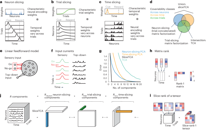
Definition of the sliceTCA modelMatrix rank and matrix factorization

Consider a data matrix consisting of N neurons recorded over T samples (time points): \(}}}\in }}^\). Matrix factorization methods find a low-rank approximation \(\hat}}}}\) following equation (1), in which each component is a rank-1 matrix: X(r) = u(r) ⊗ v(r), where \(}}}}^\in }}^\) and \(}}}}^\in }}^\) are vectors representing the neural and temporal coefficients, which are chosen to minimize a loss function. In other words, the activity of neuron n at time t is given by

$$}_=\mathop\limits_^_^_^$$

(2)

A common choice of loss function is the MSE:

$$}}}=\frac}}}-\hat}}}}\right\Vert }_^$$

(3)

Constraints may be added to the minimization of the loss, such as non-negativity of the coefficients in NMF.

Slice rank and sliceTCA

A d-tensor is a generalization of a matrix to d legs (that is, a data matrix is a 2-tensor). Here, we are specifically concerned with 3-tensors typically used in neuroscience, in which the three legs represent neurons, time and trial/condition: \(}}}\in }}^\). SliceTCA extends the matrix factorization in equation (1) by fitting X with a low ‘slice rank’ approximation23. A slice-rank-1 d-tensor is an outer product of a vector and a (d − 1)-tensor. For the 3-tensors that we have been considering, this corresponds to the outer product of a ‘loading’ vector and a 2-tensor, thus making this 2-tensor a ‘slice’ of this slice-rank-1 tensor up to a scalar multiple determined by the loading vector.

Each sliceTCA component can be one of three different slice types. For example, a neuron-slicing component can be written as X(r) = u(r) ⊗ A(r), where \(}}}}^\in }}^\) is the time-by-trial slice representing the weights of the component across both time and trials and the vector u(r) represents the neural loading vector. Components of other slice types can be constructed similarly with their respective loading vectors and slices: \(}}}}^\in }}^,\;}}}}^\in }}^\) for the time-slicing components and \(}}}}^\in }}^,\;}}}}^\in }}^\) for the trial-slicing components. Put together, this results in a decomposition of the following form:

$$}_=\mathop\limits_^_}}}}}_^_^+\mathop\limits_^_}}}}}_^_^+\mathop\limits_^_}}}}}_^_^$$

(4)

Because of the different slice types, each sliceTCA model can be described by the hyperparameter three-tuple R = (Rneuron, Rtrial, Rtime), defining the number of neuron-, trial- and time-slicing components, for a total of Rneuron + Rtrial + Rtime components.

Relationship to TCA

The extension of matrix factorizations to TCA is based on a different definition of tensor rank, in which a rank-1 tensor is as an outer product of d vectors. Each component is defined by a set of vectors corresponding to neuron, time and trial coefficients \(}}}}^\in }}^, }}}}^\in }}^,}}}}^\in }}^\) for each component: X(r) = u(r) ⊗ v(r) ⊗ w(r). Then, each element of the approximated data tensor can be written as

$$}_=\mathop\limits_^_^_^_^$$

(5)

In other words, a TCA component is a special case of a sliceTCA component in which the slice is a rank-1 matrix. In this way, sliceTCA is more flexible than TCA, as it has fewer constraints on the type of structure that is identified in the data. However, this increase in flexibility comes with the cost of an increased number of parameters, as sliceTCA fits all the entries of each slice. The flexibility of sliceTCA also leads to different invariance classes as discussed below. Finally, we note that the two methods can, in principle, be merged by incorporating TCA components into equation (4).

SliceTCA invariance classesTransformations within a slice type

Matrix factorization methods are known to be invariant to invertible linear transformations, including, but not limited to, rotations of the loading vectors. For example, suppose we decompose a matrix \(}}}\in }}^\) into a product of a matrix of weights, \(}}}\in }}^\), and a matrix of scores, \(}}}\in }}^\). Consider any invertible linear transformation \(}}}\in }}^\). Then, Y can be rewritten as

$$}}}=}}}=}}}}^}}}}}}}=\tilde}}}}\tilde}}}}$$

(6)

where \(\tilde}}}}=}}}\) and \(\tilde}}}}=}}}}^}}}}}}}\). As a result, matrix decompositions, such as factor analysis, lead to not one solution but rather an invariance class of equivalent solutions. Note that PCA avoids this problem by aligning the first component to the direction of the maximum projected variance, as long as the eigenvalues of the covariance matrix are distinct. However, other methods that do not have a ranking of components are not able to use the same alignment. SliceTCA inherits this same invariance class, as all the loading vectors within a given slice type can be transformed in the same way as equation (6) to yield the same partially reconstructed tensor for each slice type (Extended Data Fig. 5a).

Transformations between slice types

SliceTCA has an additional invariance class due to the fundamental properties of multilinear addition. For example, consider a slice-rank-2 tensor \(}}}\in }}^\), which is made of two components of different slice types. We will assume without loss of generality that these are neuron- and time-slicing components with corresponding slices V and U, such that

Then, the following transformation can be performed for the arbitrary vector \(}}}\in }}^\):

$$\begin_&=&__+__+___-___\\ &=&_\left(_-__\right)+_\left(_+__\right)\\ &=&_}_+_}_\end$$

where \(\tilde}}}}=}}}-}}}\otimes }}}\) and \(\tilde}}}}=}}}+}}}\otimes }}}\) are transformations of the original slices. This invariance class, therefore, corresponds to passing a tensor-rank-1 tensor between two slices of differing slice types (Extended Data Fig. 5b).

Note that two classes of transformations (within slice type and between slice type) commute (see proposition 2.1 of Supplementary mathematical notes); therefore, one cannot obtain a new transformation by, for example, applying the first transformation, followed by the second and then the first again.

Identification of a unique sliceTCA decomposition

To find a uniquely defined solution, we can take advantage of the natural hierarchy between the two invariance classes. Specifically, let us first define the partial reconstruction \(}}}}}^}}}}\) of the low-slice-rank approximation \(\hat}}}}\) based on the neuron-slicing components; that is

$$}}}}}^}}}}=\mathop\limits_^_}}}}}}}}}^\otimes }}}}^$$

and let \(}}}}}^}}}}\) and \(}}}}}^}}}}\) be similarly defined, so that \(\hat}}}}=}}}}}^}}}}+}}}}}^}}}}+}}}}}^}}}}\). Now, note that the within-slice-type transformations change the weights of the loading vectors and slices of all components of a given slice type without changing the partial reconstructions for each slice type. For example, applying these transformations to the neuron-slicing components would change u(r) and A(r) but not \(}}}}}^}}}}\). On the contrary, the between-slice-type transformations change the partial reconstructions \(}}}}}^}}}},\;}}}}}^}}}}\) and \(}}}}}^}}}}\), but not the full reconstruction \(\hat}}}}\). Therefore, the key to identifying a unique solution is first to perform the between-slice-type transformations to identify the unique partial reconstructions \(}}}}}^}}}},\;}}}}}^}}}}\) and \(}}}}}^}}}}\) and then perform the within-slice-type transformations to identify the unique loading vectors and components.

We leveraged this hierarchy to develop a post hoc model optimization into three steps, each with a distinct loss function. The first step identifies a model that minimizes a loss function \(}}}}_\) defined on the full reconstruction (Extended Data Fig. 8c(i)), resulting in the approximation \(\hat}}}}\). Next, because of the two invariance classes, there is a continuous manifold of solutions with different parameters (loading vectors and slices) that, after being recombined, all result in the same \(\hat}}}}\) and, therefore, have the same loss. Next, we use stochastic gradient descent to identify the between-slice-type transformation that minimizes a secondary loss function \(}}}}_\), which fixes \(}}}}}^}}}},\;}}}}}^}}}}\) and \(}}}}}^}}}}\) without affecting \(\hat}}}}\) (Extended Data Fig. 8c(ii)). Finally, we identify the within-slice-type transformation that minimizes a tertiary loss function \(}}}}_\) to arrive at the final components (loading vectors u(r), v(r), w(r) and slices A(r), B(r), C(r)) without affecting \(}}}}}^}}}},\;}}}}}^}}}}\) and \(}}}}}^}}}}\) (Extended Data Fig. 8c(iii)). Each of the three loss functions can, in principle, be chosen according to the constraints or normative assumptions most relevant to the question at hand.

We note that, if we performed only the \(}}}}_\) optimization step, then different initializations would lead to different solutions for the coefficients. Both the \(}}}}_\) and \(}}}}_\) steps are necessary to identify a unique solution across the two invariance classes. If we applied only \(}}}}_\) after \(}}}}_\), there would be no guarantee that \(}}}}}^}}}}\) would be the same for two seeds, as they could differ by more than just a rotation due to the between-slice-type invariances; therefore, it would not necessarily be possible to identify a unique solution. If we then applied \(}}}}_\) to correct this, we would need to reapply \(}}}}_\) to come up with a unique set of coefficients. Therefore, the most natural way to identify a unique solution is to exploit the hierarchical structure of the invariances by optimizing the invariances in the proposed order: \(}}}}_\), then \(}}}}_\), then \(}}}}_\). More precisely, we prove that, if each of these objective functions leads to a unique solution, the decomposition is unique under weak conditions (see theorem 2.7 in Supplementary mathematical notes).

This procedure can also be understood more intuitively by considering the case in which there is only a single component type, in which case sliceTCA reduces to a matrix factorization. Even then, minimizing \(}}}}}}}}_}}}}\) is not sufficient to determine a unique model due to there being a continuum of factor rotations that yield the same \(\hat}}}}\). PCA solves these invariances by constraining the factors to be orthogonal and ranking them by variance explained, resulting in a unique solution (under certain weak conditions, for example, up to sign reversals if all singular values are unique). This can be written through an additional loss function (equivalent to \(}}}}_\) in our framework). When considering mixed slice types, the second step (minimizing \(}}}}_\)) becomes necessary owing to the invariant transformations between slice types.

Model selection, optimization and fitting

To fit sliceTCA for a given dataset arranged as a 3-tensor, we followed the data analysis pipeline described in the main text. Below, we provide details and hyperparameters for the steps involved in the pipeline.

Fitting sliceTCA with stochastic gradient descent

For a fixed choice of R, model parameters (that is, the loading vectors and slices of all components) were fitted using the optimizer Adam54 in Pytorch. Initial parameters were randomly drawn from a uniform distribution over [−1, 1] or [0, 1] for unconstrained and non-negative sliceTCA, respectively. Throughout, we optimized the MSE loss in equation (3) with a learning rate of 0.02. Note that, during model selection, some of these entries will be masked (that is, not be summed in the loss) for cross-validation (see the next section). To introduce stochasticity in the computation of the gradient, and thus avoid local minima, we additionally masked a fraction of tensor entries so that they are not included in the calculation of the loss. This fraction starts at 80% and decreases exponentially during training with a decay factor of 0.5 over three (Fig. 2) or five blocks of iterations (Figs. 4 and 5). Within each block, the mask indices are randomly reinitialized every 20 of a total of 150 (Fig. 2), 200 (Fig. 4) or 100 iterations per block (Fig. 5). Run time scales approximately linearly with the number of components (Supplementary Fig. 16). To obtain an optimal model under a given R, we repeated the fitting procedure ten times with different random seeds and chose the model with the lowest loss.

Cross-validated model selection

To choose the number of components in each slice type, we run a 3D grid search to optimize the cross-validated loss. In addition to the decaying mask used during model fitting, we masked 20% of the entries throughout the fitting procedure as held-out data. These masked entries were chosen in randomly selected 1-s (Fig. 4) or 150-ms blocks (Fig. 5) of consecutive time points in random neurons and trials. Blocked masking of held-out data (rather than salt-and-pepper masking) was necessary to avoid temporal correlations between the training and testing data due to the slow timescale of the calcium indicator or due to smoothing effects in electrophysiological data. To protect further against spuriously high cross-validation performance due to temporal correlations, we trimmed the first and last 250 ms (Fig. 4) or 40 ms (Fig. 5) from each block; these data were discarded from the test set, and only the remaining interior of each block was used to calculate the cross-validated loss. We repeated the grid search ten times with different random seeds for train–test split and parameter initialization while keeping a constant seed for different R. Once the cross-validated grid search was complete, we selected R* by identifying the model with a minimum or near-optimal average test loss across seeds. Admissible models are defined as those achieving a minimum of 80% of the optimal performance for nonconstrained sliceTCA and 95% of the optimal model performance for non-negative sliceTCA, as compared to root-mean-squared entries of the raw data.

Hierarchical model optimization

For the first step of the model optimization procedure, we chose the MSE loss for \(}}}}_\):

$$\begin}}}_1(}},}},}},}},}},}})\\=\displaystyle\frac\left\|}}-\left(\sum\limits_ 1}^}}}}}^\otimes }}^+\sum\limits_ 1}^}}}}}^\otimes }}^+\sum\limits_ 1}^}}}}}^\otimes }}^\right)\right\|^2_F\end$$

as in the model selection (essentially refitting the model with the specific ranks identified with the cross-validation procedure on the entire data). For \(}}}}_\), we used the sum of the squared entries of the three partial reconstructions from each slice type:

$$\begin }}}_2(}},}},}})&=& \left\|}}}}}^}}-\sum\limits_}}^\otimes }}^ \otimes }}^-\sum\limits_}}^ \otimes }}^ \otimes }}^\right\|^2_F\\ &+&\left\| }}}}}^}}+\sum\limits_}}^ \otimes }}^\otimes }}^-\sum\limits_}}^ \otimes }}^ \otimes }}^\right\|^2_F\\ &+&\left\| }}}}}^}}+\sum\limits_}}^\otimes }}^\otimes }}^+\sum\limits_}}^\otimes }}^\otimes }}^\right\|^2_F \end$$

where \(}}}\in }}^_}}}}\times _}}}}\times N},\;}}}\in }}^_}}}}\times _}}}}\times T}\) and \(}}}\in }}^_}}}}\times _}}}}\times K}\). This can be thought as a form of L2 regularization. For \(}}}}_\), we chose orthogonalization and variance explained ordering through singular value decomposition (SVD).

We stress that the losses \(}}}}_,\;}}}}_\) and \(}}}}_\) may be chosen according to the specific problem at hand. For example, different factor rotations could be easily implemented into the hierarchical model optimization, including varimax or even oblique (that is, nonorthogonal) rotations. Therefore, while we chose an \(}}}}_\) that constrained components to be orthogonal, in general, sliceTCA does not necessarily need to return orthogonal components. Finally, we remark that the hierarchical model optimization procedure is valid only for unconstrained sliceTCA, as adding a non-negativity constraint restricts the possible space of solutions. This also explains why non-negative factorizations (for example, NMF) are known to suffer less from uniqueness issues but also require more complex conditions to guarantee uniqueness30. Future work could borrow from existing methods for factor rotations specifically designed for NMF to extend to non-negative sliceTCA55.

Model similarity

To estimate whether solutions found with sliceTCA are unique in practice, we adopted a measure of the model similarity of the solutions found from different random initializations4,56. This score is based on computing the angle between a pair of vectors corresponding to the loading factors of two models after components are matched according to the Hungarian algorithm. For each pair of sliceTCA components, we unfolded the slice of each component into a vector. Then, we computed the angle between the loading vectors, the angle between the vectors resulting from unfolded slices, and their average values.

Following previous work4, we computed this modified similarity score for each of the ten randomly initialized models against the model that achieved the lowest MSE loss. We calculated (1) the overall model similarity and (2) the model similarity for each slice type, which could be an informative diagnostic tool for model optimization in future work. To establish a baseline chance level of similarity, we also computed a shuffled model similarity score: for each slice type and component, we shuffled the elements of the weight vectors of one of the two models within the respective weight vectors before computing their similarity score. We then calculated the mean similarity over 100 shuffle repetitions for each slice type.

Feedforward model of perceptual learning

We modeled a population of linear neurons receiving a sensory input from upstream sources representing a go stimulus and a no-go stimulus, as well as an input representing a top–down modulation that varied from trial to trial. On each trial k, either the go or no-go stimulus was activated, with probability P = 0.5 of presenting the same stimulus as in the previous trial. Go/no-go inputs (xgo, xno) were assumed to follow the same bell-shaped activation function \(_=^^}\) on the trials during which their corresponding stimulus was presented, that is, \(_^}}=_\) if k was a go trial and \(_^}=0\) otherwise (and vice versa for the no-go input).

The stochastic learning process of the go and no-go weights \(}}}}_^},}}}}_^}\in }}^\) over trials was modeled as an Ornstein–Uhlenbeck process, which was initialized at \(}}}}_^}=}}}}_^}=\bf\) and evolved independently across neurons:

$$\begin}}}}}}_^}&=&(\boldsymbol) }}}}\left(^}-}}}}}_^}\right)}k+\sigma }}\mathbf}}}}}_\\ }}}}}}_^}&=&(\boldsymbol)}}}}\left(^}-}}}}}_^}\right)}k+\sigma }}\mathbf}}}}}_\end$$

where \(_ \sim }}}([0.2,0.8])\) are the neuron-specific learning rates, and μgo = 2, μno = 0, σ = 1.3. Furthermore, to keep weights non-negative and simulate their saturation, we clamped them to [0, 2]. The process was evaluated using a stochastic differential equation solver and sampled at K evenly spaced points in [0, 10] representing K trials.

Top–down modulation was modeled as a rectified Gaussian process:

$$_^}=\max (0,\gamma (t)),\quad \gamma \sim GP(0,\kappa )$$

with the temporal kernel:

$$\kappa (_,_)=\exp \left(-\frac_-_)}^}^}\right)$$

where \(l=\sqrt\). Top–down weights were nonplastic and distributed as \(_^} \sim }}}([0,1])\).

The activity of each neuron was thus given by

$$\begin_&=&_^}_^}}+_^}_^}+_^}_^}\\ &=&_^}_+_^}_^}\end$$

where the sensory input is combined into \(_^}=_^}}}_^}+_^}(1-}}_^})\), where \(}}^}\) is an indicator function that is 1 when trial k is a go trial and 0 if it is a no-go trial. By construction, the tensor X has a slice rank of 2, as it can be written in the following form:

$$}}}=}}}}^}}}}+}}}}^}}}}$$

where \(_^}}=_^}_\) is a time-slicing component representing the weighted, trial-specific sensory input and \(_^}=_^}_^}\) is a neuron-slicing component representing top–down modulatory factors that vary over trials. In our simulations, we used K = 100, T = 90, N = 80.

We fitted sliceTCA with non-negativity constraints to the synthetic dataset, using five blocks of 200 iterations each with a learning rate that decayed exponentially over blocks from 0.2 to 0.0125 and a mask that decayed exponentially over blocks from 0.8 to 0.05. Masked entries changed randomly every iteration. Initial parameters were drawn uniformly over [0, 1].

RNN model of condition-dependent neural sequencesModel description

We built a model of a linear RNN that produces recurrently generated sequences for different task conditions while also receiving condition-independent inputs. To generate sequences, we parameterize the connectivity matrix \(W\in }}^\) by a Schur decomposition24. Additionally, we let the central matrix have a block-diagonal structure to embed multiple sequences into the dynamics. Formally, we let W = USUT, where U is a unitary matrix and S is defined in block structure as

$$S=\left[\begin(\lambda +\epsilon )_-\lambda I&}}}\\ }}}&(\lambda +\epsilon )_-\lambda I\end\right]$$

where \(I\in }}^\) is the identity matrix and \(_\in }}^\) is the matrix with ones along its subdiagonal. The unitary matrix U was generated as the left singular vector matrix of a random normal matrix.

Each block of S corresponds to the sequential dynamics for one of the two noninterfering sequences. The specific sequence is selected by the initial state of the network. This is parameterized through the first and (N/2 + 1)th columns of U (that is, U1 and UN/2+1), which correspond to the beginning of each sequence. The RNN also receives a 2D input that is condition independent. To avoid interference with the sequences, we mapped the input through the (N/2)th and the Nth columns of U (that is, UN/2 and UN), as these are the elements corresponding to the end of the sequence. In this way, we were able to generate RNN dynamics that produce condition-specific sequences while also being influenced by condition-independent inputs.

To test the effects of different sources of noise, we considered RNN dynamics that are governed by stochastic differential equations. On trial k, the population activity \(}}}}^(t)\in }}^\) and inputs \(}}}}^(t)\in }}^\) evolve according to

$$\left\}}}}}^=(-}}}}^+W\phi (}}}}^)+B}}}}^)}t+_}}}}}_^ &}}}}^(0)=_^_+_^_\\ }}}}}^=^}}}}^}t+_}}}}}_^ &}}}}^(0)=}}}}_^\end\right.$$

where \(B=[_,_],\;_ \sim }}}(0,1/2)\) and dWi are infinitesimal increments of a Wiener process. Furthermore, we took \([_^,_^]=[\cos (^),\sin (^)]\), where θ(k) represents the angle of the task variable. In our simulations, we used K = T = N = 200 and took ϕ = id.

RNNs have three natural sources of noise: (1) noise at the level of the dynamics of each neuron, σ1dW1, which we call intrinsic noise; (2) input noise, σ2dW2; and (3) observation noise added to the full tensor, Y = X + η, where \(}}}}_ \sim }}}(0,_)\). Thus, by systematically varying σ1, σ2, σ3, we can vary the magnitude of different sources of noise in the data. Importantly, they have the property that for ϕ = id, \(}[}}}\;]=}}}\), where y(k)(t) is the activity with σi ≠ 0 for at least one i and x(k)(t) is the activity with σi = 0 for all i.

To evaluate the effect of these different sources of noise on sliceTCA, we considered the variance explained \(\kappa =1-| | \hat}}}}-}}}| _^/| | }}}-\bar| _^\) as a function of the noise level \(\zeta =| | }}}-}}}| _^/| | }}}-\bar| _^\), where \(\hat}}}}\) is the reconstruction from sliceTCA fit on Y. In the normalization term above, \(\bar\in }\) is the average over all NTK entries of Y (but we note that different marginalizations are possible57). An optimal denoiser (that is, for which \(\hat}}}}=}}}\)) would yield κ = 1 − ζ. Meanwhile, a model that fully captures the variability (including noise) in the data (that is, \(\hat}}}}=}}}\)) would have κ = 1.

Statistics and reproducibility

As we reanalyzed existing data, no statistical method was used to predetermine sample sizes. Instead, we demonstrated the utility of sliceTCA by choosing three previously published datasets representing a typical range of numbers of recorded neurons, time points and trials. For the application of sliceTCA to these example datasets and subsequent analyses, we randomly selected an example session and animal for each dataset. General trends were confirmed by fitting sliceTCA on other example sessions of the same dataset (not shown). To ensure reproducibility, we have made available the datasets for the sessions analyzed in this paper, along with the analysis code (see the ‘Data availability’ and ‘Code availability’ sections below). Model selection was performed as described in the ‘Model selection, optimization and fitting’ section above. During cross-validation, tensor entries (indexed by neurons, trials and blocks of time) were randomly allocated (80–20%) into training versus held-out data using a pseudo-random number generator. No blinding was performed, as our method is unsupervised and was applied to the full dataset. The investigators were not blinded to outcome assessment. Unless otherwise specified, we performed two-sided nonparametric statistical tests. In Extended Data Fig. 10d, model assumptions were not tested before performing analyses of variance. In dataset 3, we excluded neurons with low firing rates (<0.2 Hz); otherwise, no data were excluded from the analyses.

Dataset 1 of motor cortical recordings during a center-out and maze reaching taskDescription of the dataset

We analyzed a dataset of motor cortical (M1, n = 90) and premotor cortical (PMd, n = 92) electrophysiological recordings17. The dataset is curated and publicly available as part of the ‘Neural Latents Benchmark’ project58. Briefly, monkeys were trained to perform a delayed center-out reach task to one of 27 locations in both the maze condition (in which barriers were placed on the screen, leading to curved optimal reach trajectories) and the no-maze condition with matched target locations (classic center-out task leading to straight optimal reach trajectories). The go signal for movement initiation appeared 0–1,000 ms after target onset and 1,000–2,600 ms after the trial started with a fixation cue. We analyzed data from one animal (monkey J) in a single session and randomly subselected 12 target locations, resulting in K = 246 single-target trials in the maze reach conditions and K = 265 single-target trials in the 12 center-out reach conditions with matched target locations.

Additional preprocessing

We calculated firing rates for bins of 10 ms, which we then smoothed with a Gaussian filter with σ = 20 ms and rescaled to minimum and maximum values of 0 and 1 over the course of the experiment for each neuron separately. We selected a time period starting 1 s before movement onset (thus including a substantial part of the motor preparation period) and ending 0.5 s after movement onset when the monkey had successfully reached the target position in most trials. We did not time-warp the data. The resulting data tensor had dimensions of N = 182, T = 150 and K = 511.

Supervised mapping of neural population activity onto kinematic data

To identify the neural subspace from which 2D hand trajectories could be read out (Fig. 2a), we used ordinary least squares (OLS). Specifically, we found weights that project the neuron-unfolded data from the full neural space onto a 2D subspace that best maps onto (x, y) hand velocity with a time delay of 100 ms to account for the lag between neural activity and movement. When testing the decoding analysis after dimensionality reduction, we instead applied OLS to the reconstruction (or partial reconstruction (that is, from a single slice type)) after reshaping it into an N × KT matrix. We also used OLS to project time-averaged pre-movement activity onto target locations (Fig. 2g). For Fig. 2h, we used LDA to identify the dimension that best separates pre-movement averaged activity in clockwise versus counterclockwise curved reaches in the maze condition. To plot activity in a 3D neural subspace that contained information about the upcoming movement, we then orthogonalized the two axes that map neural activity onto target locations to the axis that distinguishes clockwise and counterclockwise movements.

For all decoding analyses, we calculated R2 values on left-out trials in a fivefold cross-validation procedure performed on 20 permutations of the trials. Decoding was performed on data from the period spanning 250 ms before to 450 ms after movement onset. For trial-resolved data (Fig. 2a, raw data, neuron-slicing NMF, TCA, trial-slicing NMF), we averaged trial-wise R2 values; for pre-movement information on target positions, we calculated a single R2 value across trials for center-out and maze reaching conditions. For trial-averaged data (Fig. 2a, trial-averaged raw data), we performed twofold cross-validation by averaging hand and neural trajectories separately for each fold and then calculating R2 values averaged over conditions and folds.

Visualization of sliceTCA weights

The results of fitting non-negative sliceTCA are shown in Fig. 2c,d and Supplementary Fig. 3. Each component consists of a weight vector and a slice of corresponding weights on the other two variables. Along the trial dimension, we sorted trials by the angle of the target position and whether trials belonged to center-out or maze reaching conditions. Along the neuron dimension of trial-slicing components, neurons were sorted by the peak latency of neural activity in the first component. For the time-slicing component, neurons were sorted according to their mean activity in the first reaching condition.

Correlation matrices

To assess the encoding similarity of movement preparation in the time-slicing component, we calculated the K × K correlation matrix of the neural encoding weights (that is, the rows of the slice in Fig. 2d) for different pairs of trials, separately for center-out and maze reach conditions, and for the PMd (Fig. 2f) and M1 (Extended Data Fig. 4c). We sorted the resulting correlation matrices by the angle of the target location (Fig. 2f).

Dataset 2 of cortico-cerebellar calcium imaging during a motor taskDescription of the dataset

We analyzed recently published calcium imaging data consisting of simultaneously recorded cerebellar granule cells (n = 134) and premotor cortical L5 pyramidal cells (n = 152) from a head-fixed mouse performing a motor task in which a manipulandum had to be moved forward and leftward or rightward for a reward18. After a correct movement was completed, a water reward was delivered with a 1-s delay, followed by an additional 3.5-s intertrial interval. Left versus right rewarded turn directions were alternated without a cue after 40 successful trials. We analyzed data from one session of a mouse in an advanced stage of learning, comprising a total of K = 218 trials. The data were sampled at a 30-Hz frame rate. Calcium traces were corrected for slow drifts, z-scored and low-pass filtered18.

Additional preprocessing

Owing to the freely timed movement period, we piecewise linearly warped data to the median interval lengths between movement onset, turn and movement end. The remaining trial periods were left unwarped and cut to include data from 1.5 s before movement onset until 2.5 s after reward delivery, resulting in a preprocessed N × T × K data tensor with N = 286, T = 150 and K = 218.

Visualization of sliceTCA weights

In Fig. 4b,c, we show the results of a fitted sliceTCA model. We further reordered trials in the trial–time slices according to trial type and neurons in the neuron–time slices according to the peak activity in the first trial-loading component. This allows for a visual comparison of the tiling structure across components. We used Mann–Whitney U tests on the time-averaged activity between reward and trial end in the trial–time slices. We used LDA to determine the classification accuracy for neuron identity (cerebellum versus cortex) based on the loading vector weights of the three neuron-slicing components found by sliceTCA. We similarly reported the classification accuracy of trial identity (error versus correct, left versus right) based on the loading vector weights of the trial-slicing components.

Matrix rank of slices

To determine whether sliceTCA finds components with higher matrix ranks compared to methods that do not demix slice types (neuron-slicing PCA and factor analysis with neuron loadings, neuron- and time-concatenated PCA and factor analysis with trial loadings), we performed SVD on the six slices (after centering) of the sliceTCA model shown in Fig. 4b, as well as on the scores of either trial-slicing or neuron-slicing PCA and factor analysis, after refolding the resulting scores into N × T or K × T matrices, respectively. We then compared these to the spectra of squared singular values obtained from the slices of the trial-slicing (Fig. 4e) or neuron-slicing components (Supplementary Fig. 8). Factor analysis was performed using the ‘sklearn’ Python package59, which uses an SVD-based solver. For comparability with PCA and sliceTCA solutions, no factor rotations were performed.

Manifolds from sliceTCA reconstructions

To analyze the geometry of neural data, we reconstructed the low-slice-rank approximation of neural activity from the sliceTCA model separately for the cerebellum and premotor cortex. We then used LDA on both raw and reconstructed data to find the three axes that maximally separate left versus right correct trials between movement onset and reward (axis 1, Fig. 4g), movement onset time versus the time of reward in all correct trials (axis 2), and the time of reward versus post-reward (axis 3). We orthonormalized the three axes and projected raw and reconstructed data onto the new, 3D basis (Fig. 4h).

We then measured the distance ratio to compare the distance between trials of the same class versus the distance between trials of distinct classes (left versus right) in the full neural space. For the reconstructed versus the full dataset, we averaged neural activity over a 650-ms window centered at movement onset and measured the Euclidean distance of the population response in each trial to the trial-averaged population response in its own trial type, compared to the Euclidean distance to the average population response of the respective other trial type: Δbetween/Δwithin, where \(_}}}}=(_^},}^})\) is the Euclidean distance between population vectors in each left trial to the mean population vector across all left trials (and vice versa for right trials), and \(_}}}}=}(_^},}^)\) is the Euclidean distance of population vectors in each left trial to the mean population vector across all right trials (and vice versa for right trials).

Dataset 3 of electrophysiology across many brain regions during perceptual decision-makingDescription of the dataset

The third analyzed dataset comprised recently published multiregion Neuropixels recordings (n = 303) in mice performing a perceptual decision-making task53. In the task, mice were presented a grating patch image with varying contrast (0%, 25%, 35%, 50% or 100%), shown on the left or right sides of a screen. The mice were trained to move the image to the center of the screen using a steering wheel within a 60-s period to receive a sugary water reward. A correct response was registered if the stimulus was moved to the center, whereas an incorrect response was recorded if the stimulus was moved to the border of the screen. We selected a single example mouse (subject CSHL049 from the openly released electrophysiology data repository).

Additional preprocessing

We binned single-neuron spiking events in 10-ms windows. Owing to the variable response times across trials, we piecewise linearly warped data between stimulus onset and reward delivery or timeout onset to correspond to the median interval length and clipped the trial period to start 1 s before stimulus onset and to end 2 s after reward delivery or timeout onset. We smoothed data with a Gaussian filter with σ = 20 ms and rescaled the activity of each neuron to a minimal and maximal value of 0 and 1 over all trials. We excluded neurons with mean firing rates below 0.2 Hz, leading to a total of n = 221 neurons analyzed of n = 303 neurons recorded. Brain regions included the visual cortex (anterior layers 2/3, 4, 5, 6a and 6b as well as anteromedial layers 2/3, 4, 5 and 6a; n = 85 neurons), hippocampal regions CA1 (n = 32 neurons) and dentate gyrus (molecular, polymorph and granule cell layers; n = 21 neurons), thalamus (including the posterior limiting nucleus and lateral posterior nucleus; n = 18 neurons) and the anterior pretectal and midbrain reticular nucleus (anterior pretectal nucleus, n = 22 neurons; midbrain reticular nucleus, n = 35 neurons) of the midbrain. In total, the resulting data tensor had dimensions of N = 221, T = 350 and K = 831.

Visualization of sliceTCA weights

In Fig. 5b, we scaled the rows of the neuron–time slices to a [0, 1] interval to highlight differences in the timing of peak activity between neurons. We then reordered neuron–time slices by the peak activity within each region for each slice type separately to show characteristic differences between neural correlates of behavioral variables. Trial–time slices were regrouped by trial type to show region-specific representations of task variables. Finally, neuron–trial slices were reordered by the average weights across the first 100 trials for each neuron within a region.

Reconstruction performance and component weights

For each neuron, we estimated the goodness of fit of the sliceTCA reconstruction as

$$1-\frac__-}_\right)}^}__^}}$$

We then quantified the contribution of the neuron-slicing components on the total sliceTCA reconstruction for each neuron n as the following ratio:

$$_^}}}}=\frac_}_^}}}}}_}_}$$

where \(}}}}}^}}}}\) describes the partial reconstruction of the data tensor from only the neuron-slicing components. We similarly defined the contributions of the time- and trial-slicing components to the sliceTCA reconstruction of each neuron n as \(_^}}}}\) and \(_^}}}}\).

Reporting summary

Further information on research design is available in the Nature Portfolio Reporting Summary linked to this article.