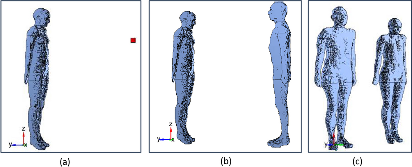
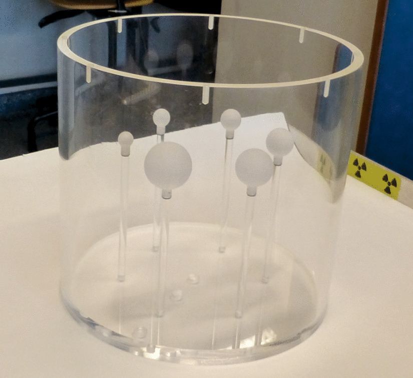
Three different configurations have been considered in this benchmarking study (Fig. 1):

a)

The ambient dose rate equivalent Ḣ*(10) was calculated 1 m away from the NM patient, represented by the reference female computational phantom of the International Commission on Radiological Protection (ICRP) [9]. For 99mTc (who has the lowest gamma emission energy of 140 keV from the 3 isotopes considered), Ḣ*(10) was also calculated at 30 cm and 50 cm from the patient (Fig. 1a).

b)

The effective dose rate Ė of an individual of a critical group was determined in a position facing the patient model at 1 m. For 99mTc, Ė was also calculated at 30 cm and 50 cm from the patient (Fig. 1b).

c)

The effective dose rate Ė of an individual of a critical group was determined in a position aside the patient model at 1 m. For 99mTc, Ė was also calculated at 30 cm and 50 cm in this configuration (Fig. 1c).

Fig. 1

MC geometry of Ḣ*(10) in a point (a), Ė for a model of an exposed individual, facing (b) or aside (c) the NM patient. The NM patient model is represented by the ICRP reference female computational voxel model [9]. The exposed individual is represented alternatively by the ICRP reference female and male (only shown in the figure) computational voxel models to calculate sex-averaged effective doses

The benchmarking study was performed for typical clinical procedures: 99mTc-HDP/MDP (Hydroxymethylene diphosphonate /Methylene diphosphonate), 18FDG (2-Deoxy-2-[18F]fluoroglucose) and Na131I (Sodium iodide).

Biokinetic models and time activity curves for 99mTc-HDP/MDP, 18F-FDG and Na131I

For 99mTc-HDP/MDP, the biokinetic data early published in ICRP Publication 53 [6] and later adopted by ICRP Publication 128 [10] was used in this study. The time activity curves in the source regions (Table 1) were calculated analytically using biokinetic data. Urinary excretion in the bladder is calculated separately according to Snyder and Ford [22]. Also for Na131I, the current ICRP biokinetic model in Publication 128 [10] was used in the present work for the source regions presented in Table 1. The compartmental model for 18FDG which was recently developed by an ICRP task group [15] was applied. The time activity curves in the source regions indicated in Table 1 were calculated using the software SAAM II (Nanomath (LLC), Spokane, WA, USA). To model the urinary excretion rate of patients in a realistic way, for these three given radiopharmaceuticals, the information of patient bladder voiding time obtained from the ambient dose rate measurement data at 1 m from NM patients was used in the modelling. These measurement data are described in one of the following subsections of this paper.

Table 1 Radiopharmaceuticals and source regions

For the 3 given radiopharmaceuticals, calculations of the time activity curves in corresponding source regions were performed independently by different groups of scientists and benchmarked against each other. For 99mTc-HDP/MDP and Na131I it was evaluated if the integrals of time activity curves were in agreement with the ICRP values.

Monte Carlo simulations

In the Monte Carlo simulations, the organs of the patient model are defined as radioactive source regions, while the tissues of the exposed individual model(s) are defined as target tissues, i.e. tissues used to score energy depositions and thus their absorbed doses. For the source modelling, the biokinetics of the 99mTc-, 18F- and 131I-based radiopharmaceuticals in the different source regions are considered.

The effect of each source organ on the exposed individual is additive, therefore the simulations are performed for each source region individually. The output of the MC codes is given in Sv per emitted source particle. By considering the total emission probabilities of a given radionuclide (i.e. the number of particles emitted per second), simulated doses are converted to Sv/s/Bq. Finally, all results in this study are expressed in µSv/h/MBq.

When summing the results over all source regions, the resulting cumulated Ḣ*(10) for each time point (t) post-administration, is given by Eq. 1:

$$\dot^ \left( \right)\left( t \right) = \sum_}\;}}} }\;}}} \left( t \right)\dot^ \left( \right)_}\;}}} }$$

(1)

With

Ḣ*(10)(t): ambient dose rate equivalent per unit of administered activity at time t post administration (Sv/s/Bq).

asource region(t): fractional activity of the administered activity in the source region at time t post administration.

Ḣ*(10)source region: ambient dose rate equivalent per unit of administered activity in the source region (Sv/s/Bq)

Ė(t) of an individual is obtained as the average of the organ dose rates to both the male and female ICRP reference voxel phantoms, weighted with the ICRP-103 tissue weighting factors [8]. The cumulated effective dose rate for each time point (t) post-administration per administered activity is given by Eq. 2:

$$\dot\left( t \right) = \sum\limits_}\;}}} }\;}}} \left( t \right)\dot_}\;}}} }$$

(2)

With

Ė(t): Effective dose rate per unit of administered activity at time t post administration (Sv/s/Bq)

asource region(t): fractional activity of the administered activity in the source region at time t post administration

Ėsource region: effective dose rate per unit of administered activity in the source region (Sv/s/Bq)

The Monte Carlo simulations for both set-ups are performed with five different radiation transport codes: PHITS (version 3.2) [24], MCNP-X (version 2.6c) [26], TRIPOLI-4® [5], Geant-4 (version 11.0) [1] and GATE (version 9.2) [14] (only for 131I). The results from all codes are compared for both configurations, separately per source organ and for the cumulated Ḣ*(10) or Ė over time.

Ambient dose rate measurements

In seven different European NM departments, Ḣ*(10) measurements were performed at 1 m from the patients at different time points post-administration, with two measurements for each time point. Measurement data was obtained in six hospitals for 99mTc-HDP/MDP, in three hospitals for 18FDG, and in one hospital for Na131I. First, an intercomparison exercise of the measurement equipment was performed for 99mTc-HDP/MDP and 18FDG. In each participating hospital Ḣ*(10) were measured three times at 1 m from a 10 ml vial containing an activity calibrated with the activity meter of the local radiopharmacy laboratory. The calibrated measurement equipment of the participating hospitals is listed in Table 2, one of the three hospitals that performed measurements for 18FDG did not participate to this intercomparison exercise. The measurements are compared against a reference value, determined through Monte Carlo simulations. The fluence in a 1 mm3 air cube at 1 m from the center of the simulated vial is calculated and converted to Ḣ*(10) with the ICRP74 conversion coefficients [7]. The vial is modelled as a 50 mm high cylinder with 20 mm diameter and 1 mm wall thickness. The walls are made of borosilicate glass and the vial is half-filled with a water solution, containing the radioactive source.

Table 2 Measurement equipment for Ḣ*(10) dose rate measurements

For the ambient dose rate measurements at 1 m from the patients in the participating hospitals, patient (sex and BMI) and procedure data (radiopharmaceutical, administered activity, syringe/vial residual activity after administration, number and timing of bladder voiding, if applicable) are collected. The measurement data of each patient is corrected for the difference against the nominal value obtained from the equipment intercomparison exercise and compared against the Monte Carlo simulations performed for the set-up illustrated in Fig. 1a. For this comparison, the average of Ḣ*(10)source organ from the simulation results of all participating Monte Carlo codes was taken.

Sensitivity study on the influence of patient model morphology

To evaluate the influence of body morphology on the external dose rates from NM patients, a sensitivity study is performed calculating the ambient dose rate equivalent Ḣ*(10) at 1 m from four different computational voxel phantoms, selected from a phantom library developed by Broggio et al. [3]. Four male models are selected with a model height of 164 ± 6 cm, which is close to the height of the ICRP reference female voxel phantom used in the previous simulations, and a body mass ranging from 50 to 85 kg (Table 3).

Table 3 Body morphology of computational models used for the sensitivity study

The Monte Carlo simulations are performed with MCNPX 2.6c for the radionuclide 99mTc.

Uncertainty assessment

The following contributions to the total uncertainty on the experimental data of ambient dose rate equivalent per administered activity at 1 m from the patient have been considered:

The uncertainty of the ambient dose rate measurement device used by the specific center. This uncertainty is mainly defined by the energy and angular response from the device itself and is a priori unknown for the devices used in this study. Therefore, the average relative deviation of the different measurement devices used in the intercomparison exercise against the reference value for 99mTc is used to represent this device-related uncertainty contribution.

The positioning uncertainty of the measurement device, caused by the different sizes of the sensitive volume of the chambers used. Assuming a possible error of 10 cm in both directions along the line patient-detector at their distance of 1 m, this results in an uncertainty of ± 20%, applying the inverse square law.

The uncertainty on the activity measurement of the syringe used for patient administration. From previous national and international intercomparison studies of radionuclide calibrators [20, 21]

For the uncertainty on the simulated Ḣ*(10)(t) data, the following contributions are considered:

The absolute uncertainty on the mean value obtained from all the different MC codes for the Ḣ*(10)source organ factor in (Eq. 1) for each individual source organ.

The uncertainty on the activity values per time point for each source organ as a result of the biokinetic model parameters. Although this uncertainty is expected to be the largest of all uncertainty contributions in this study, it is very difficult to quantify it. In general, a variability by a factor of 2 or more is considered reasonable for kinetics of any given radiopharmaceutical as stated by [23] and variations of the same order of magnitude can be observed in whole-body retention curves from [16, 18] for 177Lu-based therapies. With time-activity curves considered as being log-normal, a factor 2 variability means that the activity values lie within [A(t)/2 and 2xA(t)).

The statistical uncertainty on the simulated results for each code was very small (< 1%) and therefore neglected in the total uncertainty assessment.

Following the GUM (Guide to the expression of Uncertainty in Measurement) approach [13] for combined uncertainties for quantities obtained following Eq. 1, the total uncertainty U(t) on the simulated Ḣ*(10) data is obtained as follows:

$$U\left( t \right) = \left( \left( t \right)*u\left( } \right)} \right]^ + \left[ \left( t \right)*u\left( } \right)} \right]^ + \ldots + \left[ *u\left( \left( t \right)} \right]^ + } \right[C_ *u\left( \left( t \right)} \right]^ + \ldots } \right)^ \!\mathord}\right.\kern-0pt} \!\lower0.7ex\hbox}}}$$

(3)

with u(Ci) the uncertainty on Ḣ*(10)source organ for source organ i and u(ai(t)) the uncertainty on the fractional activity in source organ i at time point t. In order to be able to apply the uncertainty propagation formula in Eq. 3, the log-normal uncertainty factor of 2 needs to be transformed into an uncertainty factor describing a normal distribution in the following way: \(u\left( \left( t \right)} \right) = a\left( t \right)\left[ \right)^ } \right] - 1} \right]^}\) using the coverage factor k = 2 for 95% confidence intervals [4].