Our hospital Medical Science Research Ethics Committee approved this study (M2019056). The twelve fresh-frozen specimens used in this study were obtained from donations to our university anatomy program and included eight left knees and four right knees. Preoperative magnetic resonance imaging (MRI) was used to exclude specimens from patients with ligament injuries or cartilage diseases. In a simulated operating room, an experienced surgeon used a robotic system (TiRobot™, TINAVI Medical Technologies Co., Ltd., Beijing, China) combined with an arthroscopic system (Smith & Nephew, Inc., Arkansas, USA) to complete the registration of the ACL insertion points, the planning of the tunnels, and the drilling of the tunnels. Postoperative 3D computed tomography (CT) was used to measure the position and length of the actual tunnel and compare them with those of the planned tunnel. Twelve consecutive patients who underwent traditional arthroscopic ACL reconstruction performed by the same surgeon in our hospital were included. The ACL bone tunnel position was measured by 3D CT postoperatively and compared with the position of the bone tunnel drilled on the specimen by the robot. Finally, the bone tunnel positions of traditional surgery and robotic surgery were compared with the ACL positions reported in the literature to verify the anatomy of the bone tunnel positions of the two surgical methods.

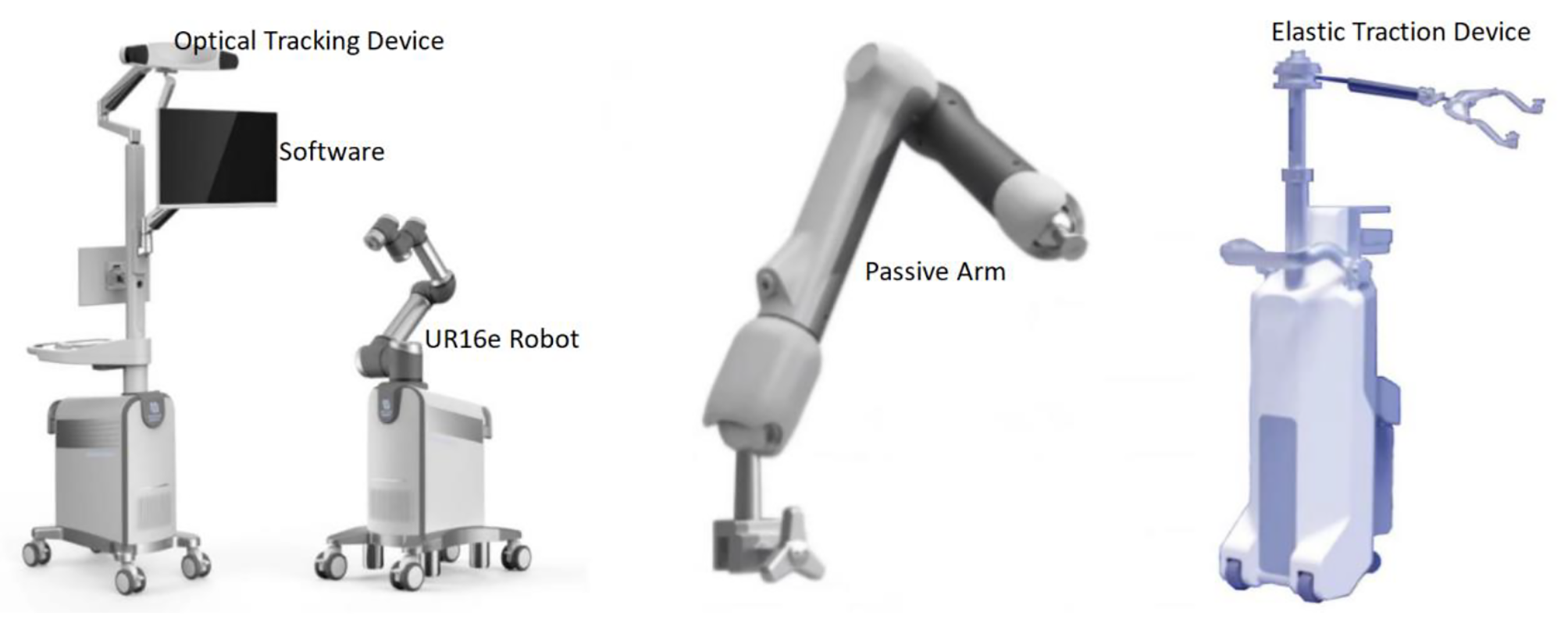
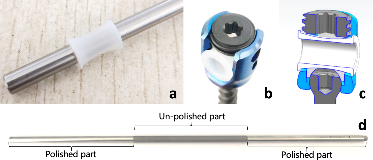
As shown in Fig. 1, the main part of the surgical robot system includes a robotic arm, a surgical planning and controlling workstation, and an optical tracking device. The surgical instruments associated with the robot system include two specially designed femoral and tibial locators for the cruciate ligament as well as femoral and tibial trackers.

The appearance and placement of each part of the robot system

The robot arm has 6 degrees of freedom and can perform automatic navigation and positioning flexibly. The workstation can plan and adjust the position of the bone tunnels according to the 3D images. The optical tracking device can track the spatial position of the patient's knee in real time. During surgery, the robot arm must be located on the same side as the surgeon, whereas the workstation and the optical tracking device must be located on the opposite side to prevent occlusion between the optical tracking device and the knee, which can affect the spatial positioning.

Each specimen was thawed for 24 h before operation. The knee was positioned flex-90°, and standard anterolateral and anteromedial approaches were then established, and an arthroscope was used to observe the integrity of the intra-articular structures. Subsequently, the femoral and tibial trackers were fixed to the anterior of the femur and tibia, respectively, 15 cm from the knee joint line, respectively.

After the trackers were fixed, the knee was straightened, placed within the robotic arm, and scanned with a 3D C-arm (Siemens, Munich, Germany). The 3D images generated after scanning were transmitted to the workstation of the robot to complete the registration of the knee and the images. The knee was subsequently placed on a rigid fixation frame with 90° flexion and arthroscopy was subsequently performed. The insertion point of the native ACL in the femur was registered by a specially designed ACL femoral locator via arthroscopy, and this insertion point was used as the exit point of the femoral tunnel. Similarly, the entrance to the femoral tunnel was registered on the lateral aspect of the lateral femoral condyle by the ACL femoral locator. The position of the locator can also be displayed on the workstation in real time when planning the tunnel (Fig. 2B). Once both exits and entrances were registered, the initial planned tunnel was automatically generated and viewed in a 3D image. At this point, the surgeon adjusted the position, angle, and length of the tunnel relative to the lateral femoral condyle according to the bony landmarks displayed in the 3D image and finally obtained a satisfactory femoral planning tunnel. Similarly, the tibial insertion of the ACL was selected as the exit of the tibial tunnel by the specially designed ACL tibial locator, and the appropriate position on the medial side of the tibia was selected as the entrance of the tibial tunnel (Fig. 2A). After the registration and tunnel adjustment, the planned tunnel of the tibia was also determined. Preoperative planning was completed after both the femoral and tibial tunnels were confirmed. The image above the workstation at this time is shown in Fig. 2C. The final planned bone tunnel generated on the 3D image is shown in Fig. 2D, E.

Preoperative planning process. A the tibial tunnel entry point planning process; B the tibial tunnel exit-point planning process; C simultaneous observation of the position of the locator in real time through imaging information provided by the doctors, in addition to the arthroscopic field of view and visual observation; D and E 3D views of the final generated femoral and tibial tunnels

The bone tunnels were drilled according to the planned tunnels generated during operation. In this process, the end of the robot arm and the trackers on the specimen must be in the field of view of the optical tracking device at all times so that the workstation can obtain the spatial position of the robot arm and the specimen in real time.

Drilling of the femoral tunnel was performed first. The ACL femoral tunnel was selected on the workstation, and the foot pedal of the robot arm was pressed to start the robot arm. During the movement of the robot arm, its position and the error between it and the planned tunnel are displayed in real time on the workstation. Finally, the robotic arm end automatically moved to the planned femoral tunnel entrance and stayed. The surgeon inserted a 2 mm Kirschner wire into the lateral femoral condyle through the guide sheath at the end of the robot arm and the ACL femoral tunnel was drilled along the Kirschner wire with an 8 mm femoral drill.

Next, the tibial tunnel was drilled. Similar to the above procedure, the surgeon selected the ACL tibial tunnel on the workstation, activated the robotic arm to achieve automatic navigation, and drilled the ACL tibial tunnel with a Kirschner wire and an 8 mm tibial drill. Figure 3A shows the tibial tunnel drilled by the surgeon with the robot arm.

Tunnel location as shown in the arthroscopic field and 3D CT images. A After the robot arm completes the positioning step, the doctor drills the bone tunnel; B the location of the intra-articular opening of the femoral tunnel on 3D CT; C the location of the intra-articular opening of the tibial tunnel on 3D CT

The patient was in the supine position with the knee in 90° flexion. During the operation, arthroscopic exploration of the knee joint cavity and debridement of the ACL stump were routinely performed. According to the surgeon's personal experience, bony landmarks were used to determine the locations of the ACL femoral and tibial tunnel openings. Traditional ACL femoral and tibial locators (Acufex, Smith & Nephew, USA) were used to determine the location of ACL insertion. Finally, Kirschner wires and 8 mm diameter bone tunnel drills were used to drill the bone tunnel.

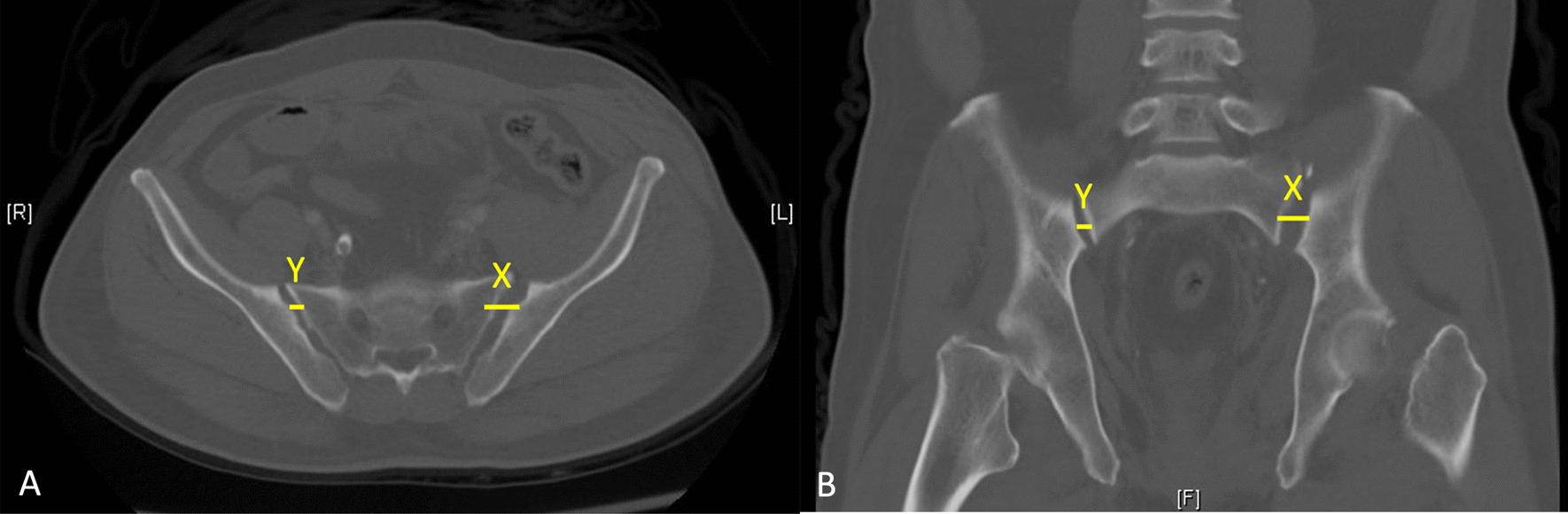
After bone tunnel drilling, 3D CT was performed to evaluate the position of the tunnels. As shown in Fig. 3B, C, the location of the tunnel is indicated by the central point of the tunnel opening in the joint. The quadrant method was used to measure the position of the femoral and tibial tunnels [26, 27]. Rectangular coordinate systems were created on the medial aspect of the lateral femoral condyle and on the tibial plateau to calculate the coordinates of the tunnels and accurately represent the location of the tunnels. The position of the femoral and tibial insertion of the ACL was determined using the studies of Anagha et al. [28] and Pisit et al. [29], respectively.

For the femur, as shown in Fig. 4A, a rectangle was established below Blumensaat’s line, and one edge representing the total sagittal diameter of the lateral femoral condyle of the rectangle was located on Blumensaat’s line. The other edge representing the height of the intercondylar notch is tangential to the posterior margin of the lateral femoral condyle. The position of the femoral tunnel is indicated by the percentage in the deep-shallow (D–S) direction and in the high-low (H–L) direction.

A tunnel positions in the femur. The green points represent the tunnel location for traditional surgery, the blue points represent the tunnel location for robotic surgery, and the red points represent the ACL insertion as described in the literature; B the mean femoral tunnel position

For the tibia, as shown in Fig. 5A, a rectangle was built on the tibial plateau with one edge which was tangent to the medial edge of the tibial plateau, parallel to the anteroposterior diameter of the tibial plateau, and the length represented the anteroposterior diameter of the tibial plateau. The other side was tangential to the anterior edge of the tibial plateau, and its length was the mediolateral diameter of the tibial plateau. The position of the tibial tunnel was indicated by the percentage in the medial–lateral (M–L) and the anterior–posterior (A–P) directions.

A Tunnel positions in the tibia. Green points represent the tunnel location for traditional surgery, blue points represent the tunnel location for robotic surgery, and the red point represents the ACL insertion as described in the literature. B The mean tibial tunnel position

The error in the bone tunnel position was calculated as the absolute value of the difference between the actual bone tunnel position and the anatomical position of the ACL, expressed as a percentage.

Based on similar previous studies [30], a sample size of 12 knees per group was considered adequate. The Shapiro–Wilk test was used to test the normality of the data. Normally distributed data are expressed as the mean ± standard deviation (SD), and a t test was used for comparisons between groups. Data that did not follow the normal distribution were expressed as median and interquartile range, and comparison between groups was performed using the Mann–Whitney U nonparametric test. SPSS version 27.0 (IBM Corp., Armonk, N.Y., USA) software was used for data analysis. Statistical significance was set at p < 0.05.