Ethics and information governance

Our work received approval from the institutional review board of Tianjin Medical University Cancer Institute and Hospital (IRB no. bc2021182). Data collection and other procedures were performed in accordance with principles of Good Clinical Practice and Declaration of Helsinki guidelines (1975, revised 1983), and with other relevant ethical regulations. All patients provided written informed consent before undergoing pathological examination. Each image was anonymized before being incorporated into the framework. Likewise, only deidentified and relabeled clinical data were used for research, without the involvement of any personal patient information.

External public datasets

For some tumors of rare origin, or those rarely metastasizing to the thoracoabdominal cavity (such as those of the nervous and bone and soft tissue systems, melanoma and head and neck tumors), the sample size of ascitic and pleural cytological smear images was limited. We acquired a large collection of pathological images from the publicly available medical dataset TCGA via the NIH Genomic Data Commons Data Portal. These data included of a wide range of tumors, both rare and common cancers, covering 32 subtypes: acute myeloid leukemia, adrenocortical carcinoma, urothelial bladder carcinoma, breast ductal carcinoma, breast lobular carcinoma, cervical cancer, cholangiocarcinoma, colorectal carcinoma, esophageal cancer, gastric adenocarcinoma, glioblastoma multiforme, head and neck squamous cell carcinoma, hepatocellular carcinoma, chromophobe renal cell carcinoma, clear cell renal cell carcinoma, papillary renal cell carcinoma, lower-grade glioma, lung adenocarcinoma, lung squamous cell carcinoma, mesothelioma, ovarian serous adenocarcinoma, pancreatic ductal adenocarcinoma, paraganglioma pheochromocytoma, prostate carcinoma, sarcoma, skin melanoma, testicular germ cell tumor, thymoma, thyroid cancer, uterine carcinosarcoma, endometrial carcinoma and uveal melanoma. In aggregate, a total of 1,360,892 image patches were clipped from whole-slide images obtained from 11,607 patients, from which the raw data amounted to approximately 20 terabytes.

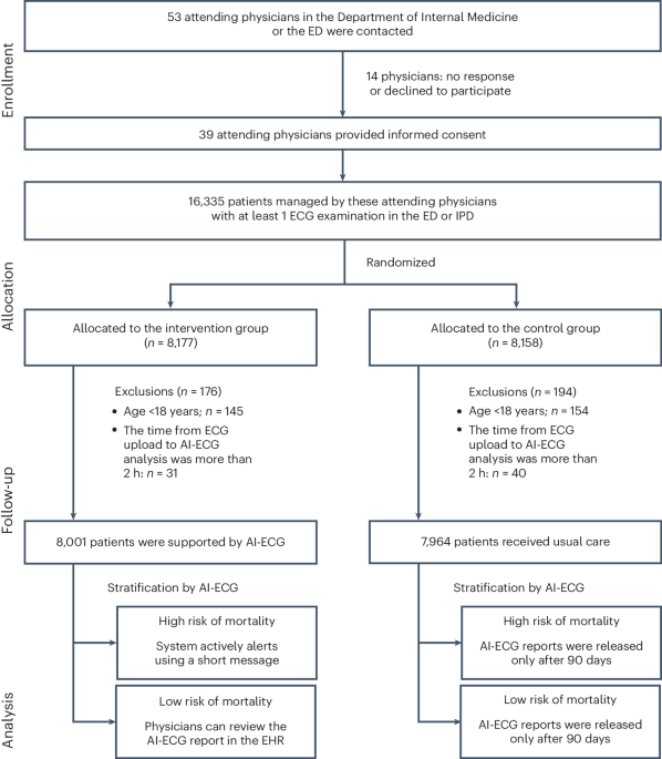
Training and testing datasets

We retrospectively collected 42,682 cases of cytological smear images from cohorts of patients who had attended three large tertiary referral institutions (Extended Data Fig. 3 and Table 1). Ultimately we enrolled 14,008 cases from Tianjin Medical University Cancer Hospital between September 2012 and November 2020, 20,820 cases from Zhengzhou University First Hospital between August 2011 and December 2020 and 7,854 cases from Suzhou University First Hospital between June 2010 and December 2020. We randomly selected 70% of these as training sets and 30% as internal testing sets. We ensured that the testing sets of patients did not overlap with those in the training set. Finally, the training sets consisted of 29,883 cases of which the three internal testing sets consisted of 12,799 cases. For ease of description we denoted these testing sets as Tianjin, Zhengzhou and Suzhou, respectively. In particular we added two independent external testing sets enrolled from Tianjin Medical University Cancer Hospital between June and October 2023 (the Tianjin-P testing set; 3,933 cases prospectively enrolled) and from Yantai Yuhuangding General Hospital between February 2013 and May 2022 (Yantai testing set; 10,605 cases retrospectively enrolled). These two external testing sets were both fully unseen cohorts that were used further to test the generalization capabilities of our model (Fig. 1).

We retrieved cytological imaging data for cells isolated from pleural and peritoneal fluid from pathologic databases. In contrast to the malignant group, the benign group consisted of patients diagnosed with benign diseases such as decompensated liver cirrhosis, nephrotic syndrome, constrictive pericarditis, pulmonary edema and pleuritis. To ensure that the diagnosis of each patient was based not only on histopathological reporting, other electronic medical records were also retrieved as ancillary verification. All pertinent clinical information—disease history, laboratory test results, family oncologic history, surgery records, endoscopic or interventional examination, chemotherapy or radiotherapy and follow-up interviews—was obtained where applicable and available. To test our model in the clinical setting scenario we divided patients into high- and low-certainty groups according to the level of supporting evidence. The high-certainty group included (1) patients whose primary tumors had been resected and with a definitive routine histopathological diagnosis and (2) patients who had undergone immunohistochemical examination by paraffin sections of cell sediment, the results of which strongly suggested the origin of malignant tumors38,45,46. The low-certainty group consisted of (1) patients whose primary or metastasized tumors merely underwent fine-needle puncture biopsy47,48 and (2) patients whose putative differential diagnosis was arrived at solely by comprehensive clinical and radiological findings. Because it is not practical to obtain a definitive ground-truth origin for some patients, with CUP, the assigned primary diagnosis of each case was reviewed by a medical team consisting of clinicians, physicians, surgeons and pathologists.

Clinical taxonomy

To guarantee the quality of each image we asked five senior pathologists (each with >15 years experience of clinical practice) to collect corresponding pathological examination results of either sediment paraffin H&E images or surgically resected or needle biopsy specimens to verify their accuracy and authenticity. Cases were excluded for which clinical diagnosis was ambiguous or the origin of the primary tumor was unknown. A final taxonomy label was assigned to each case manually by consensus among all five pathologists. Patients treated previously by palliative chemotherapy or radiotherapy (high possibility of therapy-related changes in tumor cell morphology or high false-negative rates) were excluded from both training and testing sets. The various cancer types from these patients were first grouped into 12 subgroups according to organ function and origin. Tumors originating from esophagus, stomach, duodenum, intestine, appendix, colon and rectum were grouped under cavity digestive system; similarly, tumors from the liver, gallbladder and pancreas were grouped under secretory digestive system and those from ovary, fallopian tube, corpus uteri, cervix uterus and vagina were grouped under female genital system. Meanwhile, because of the particularity and function of the mammary gland, breast cancer was grouped under female genital system. Tumors from kidney, ureter, bladder and urethra were grouped under urinary system; to remain consistent with clinical convention, tumors from prostate, testicle and seminal vesicle were also grouped under urinary system. Tumors from lung and trachea were grouped under respiratory system. Tumors from head and neck were grouped together. Tumors from the central nervous system and peripheral nervous system were categorized as one group. Bone and soft tissue tumors were also categorized as one group. For melanoma, mesothelioma and thymoma, on account of their unique growth characteristics these were grouped individually. In addition, acute or chronic leukemia and lymphoma were grouped as blood and lymphatic system. Because some tumors (such as those of the urinary system, head and neck, nervous system, bone and soft tissue, melanoma and thymoma) rarely metastasize to the chest or abdominal serous cavity, the number of cytological images available for model training from those was limited. In the current study, specimens of mesothelioma from all four institutions were also relatively scarce. We excluded these rare cytological smear images from the above cancers and further integrated the remaining 57,220 cases into five main categories: benign, digestive system (consisting of both cavity digestive system and secretory digestive system), female reproductive system (including breast cancer), respiratory system and blood and lymphatic system (Fig. 1).

Data curation and patching

In this study, cytology smear images rather than whole-slide images were retrieved from a real-world, clinical scenario. Initially pleural and abdominal fluids were extracted by fine-needle aspiration and directly prepared as smears for microscopic observation (JVC TK-C9501EC, Olympus BX51 at either ×400 or ×200 equivalent magnification). The pathologists selected between five and ten fields with concentrated tumor cells best representing the pathological features for semiqualitative analysis. The original image format stored in the database was 2,797 × 1,757 alike pixels. Due to variation in cell shape arising from the different tumor origins, as well as the relatively high proportion of background in cytological images, it is usually impossible to develop deep-learning models directly from these large images and thus we split each image into a list of patches of 224 × 224 pixels. We excluded blank, poorly focused and low-quality images containing severe artifacts. Extracted patches from the same image were located in a single package. For cancer-positive packages there must be at least one patch that includes tumor cells; for negative packages, no patch must contain tumor cells.

Development of the feature extractor

We used self-supervised feature representation learning with momentum contrast (MoCo) as learning representation for histological and cytological images. The key concept of this method is to minimize the contrastive loss of different augmented versions of a given image. The feature extractor is a 50-layer residual neural network (ResNet) consisting of four residual blocks, followed by a multilayer perceptron (MLP) to project the outputs from ResNet into a latent space where contrastive learning is performed. The use of MLP has proved to be beneficial in regard to contrastive learning. The framework of MoCo is a Siamese network consisting of two feature encoders whose parameters are denoted as θk and θq. MoCo learns similar/dissimilar representations from images that are organized into similar/dissimilar pairs, which can be formulated as a dictionary lookup problem. For a given image x we perform random data augmentation for x giving rise to xk and xq; xk is fed into θk and xq into θq. This problem can be optimized efficiently by InfoNCE loss49:

$$}}_^,\left\^\right\}}=-\log \frac^/\tau )}^}\right)+\sum _^}\exp\left(q.\frac^}\right)}$$

where q is a query representation and k+ is the representation of a similar key sample of q, both of which are obtained via data augmentation for the same image. is the set of representation of dissimilar samples of q, which are obtained via data augmentation for the other images. The size of dissimilar samples was set to 65,536. The two feature encoders, θk and θq, are updated in different ways, whereas θq is updated by back-propagation and θk is updated according to θk ← mθk + (1 − m)θq. m ∈ (0, 1) is the momentum coefficient and was set to m = 0.999 in our study. Hyperparameter τ was set to 0.07. We used stochastic gradient descent to train the network for 200 epochs with an initial learning rate of 0.015, weight decay of 1 × 10−4 and batch size of 128 on four graphics processing units. The learning rate was scheduled by cosine decaying. Specifically, the learning rate at the ith epoch was set to initial_lr × 0.5 × (1.0 + cos(π × i/n)) where n is the total number of training epochs, set to 200 in this study. The ResNet encoder is eventually used as feature extractor. Data augmentation includes random resize and crop, color jittering, grayscaling, Gaussian blurring, flipping and subsequently normalization by the mean and standard deviation of channels R, G and B. In total, 1,360,892 histological image patches from TCGA and 29,883 cytological image patches were used for the development of the histological feature extractor and cytological feature extractor, respectively. We eventually obtained two feature extractors: cytological and histological feature extractors.

For a given cytological image with n tiling patches we converted each patch into a feature vector of 1,024 dimensions. These feature vectors were then combined as feature matrix Ximage of n rows and 1,024 columns. Besides image features we took clinical parameters as inputs including age, sex and specimen sampling site. In this scenario we embedded age, sex and specimen sampling site into a vector of 1,024 dimensions, denotated as Xage, Xsex and Xlocation. The input to the attention-based MIL classifier can be set to X = Ximage and X = Ximage + Xage + Xsex + Xlocation.

Model training

Because each extracted patch represents only a small fraction of tumor features or tissue content, labeling these with patient-level diagnosis is inappropriate. We therefore used a weakly supervised machine learning method and trained a multitask neural network model named TORCH while taking into account information from the entire package. Parameters including sex, age and specimen sampling site (hydrothorax and ascites), combined with cytological images, were taken as inputs. We trained our model in an end-to-end fashion with stochastic gradient descent for 100 epochs at a constant learning rate of 2 × 10−4, weight decay of 1 × 10−5 and batch size of 1 using the Adam optimizer50. From epoch 60 and beyond, the model with the lowest validation loss was selected as the optimal model. We trained four deep neural networks individually on the training set. These networks included attention-based, multiple-instance learning (AbMIL), AbMIL with multiple attention branches (AbMIL–MB), transformer-based MIL (TransMIL) and TransMIL with cross-modality attention. These methods can be categorized as either attention- or transformer-based MILs. The objectives and differences of these four algorithms are shown in Supplementary Table 19. Image features were extracted using the cytological and histological feature extractor. For each network we trained and obtained three models for different combination of inputs: (1) cytological image features plus age, sex and specimen sampling sites; (2) histological image features plus age, sex and specimen sampling sites; and (3) cytological and histological image features plus age, sex and specimen sampling sites. As a result, we obtained 12 trained models. Finally we performed model ensembling by averaging the prediction probabilities from these models. Model training and evalutation were performed with PyTorch (v.1.12.1) on a DGX A100 computing server.

AbMIL

In the setting of multiple-instance learning, a cytological image is considered as a bag and image patches from that cytological image are instances51,52. For a cytological image with k patches we can obtain a feature matrix, denoted as [x1, x2, …, xk]T; xi is the feature vector of the ith image patch output from the feature extractor. A two-layer, fully connected neural network transforms xi into latent vector hi:

$$_=}}\left(_\right.\left(}}\left(__+_\right)\right)+_$$

where W1, W2, b1 and b2 are parameters and ReLU is the activation function. The attention weight ai for hi is defined as51

$$_=\frac_)\odot }}(U_))}_^\exp (\tanh (V_)\odot }}(U_))}$$

where V and U are weight parameters and tanh and sigmoid are activation functions. Attention pooling was applied to obtain the sample-level features:

$$\begin=^}\\}\;=\_},_},\ldots,_}}\}\;}\;H=\_},_},\ldots,_}\}.\end$$

Subsequently, a fully connected layer parameterized as W3 and b3, followed by sofmtax, was used to transform sample-level features into probabilities:

$$p=}}\left(_Z+_\right).$$

AbMIL–MB

This approach is an extension of attention-based deep MIL based on Lu et al.52. Let \(}}_\in }}^\) denote the patch-level representation extracted from the feature extractor. A fully connected layer, \(_\in }}^\), projects zk into a 512-dimensional vector hk = W1zk. Suppose the attention network consists of two layers. \(_\in }}^\) and \(_\in }}^\); subsequently the attention network splits into N parallel attention branches, \(_,_,\ldots,_\in }}^\). Then, N parallel classifiers (that is, \(_,_,\ldots, _\in }}^\)) are built to create a class-specific prediction for each cytological image. The attention score of the kth patch for the ith class ak,i is calculated as

$$_=\frac_(\tanh \left(_}}}}_\right)\odot }}\left(_}}}}_\right))\}}_^\exp \_(\tanh \left(_}}_\right)\odot }}\left(_}}_\right))\}}.$$

The aggregated representation for a cytological image for the ith class is given by

$$\displaystyle}}_}},i}=\displaystyle\mathop\limits_^_}}_.$$

The logit value for a cytological image is calculated as

Softmax function is applied to convert scyto,i into the predicted probability distribution over each class.

TransMIL

TransMIL for whole-slide image classification was investigated in our recent study53 and in a study by Wagner et al.54. For a given cytological image we first split it into multiple 224 × 224 image patches. Let \(_\in }}^\) denote the patch-level representation. A fully connected layer \(_\in }}^\) projects zk into a 384-dimensional vector hk = W1zk. Clinical features including sex, age and sample origin (that is, ascites or pleural effusion) are independently embedded into a 384-dimensional vector: hsex, hage and horigin. Similar to the vision transformer, we prepend a learnable embedding hclass to the sequence of image patches. The state of hclass at the output of the transformer encoder is used as the representation of that cytological image. We then concatenate the patch-level features with clinical features as h = . The position embeddings \(p\in }}^\) are added to h to retain positional information, giving rise to input x = h + p.

The concatenated features \(x\in }}^\) are passed through the transformer encoder, which consists of three layers, to make a diagnostic prediction. The transformer encoder layer comprises a multiheaded self-attention and a positionwise, feedforward neural network (FFN). The ith self-attention head is formulated as

$$}}_\left(_,_,_\right)=}}\left(\frac__^}_}}\right)_$$

where Qi, Ki and Vi are three matrices that are linearly projected from the concatenated feature matrix x and dk is the dimension of Qi, which is used as scaling factor. In this study dk is set to 64. Qi, Ki, Vi = LP(x), where LP represents linear projection. Multiheaded self-attention is the concatenation of different self-attention heads:

$$}}\left(Q,K,V\right)=}}\left(}}_,\ldots ,}}_\right)^$$

where Wo represents the learnable projection matrix. The pointwise FFN has two linear layers with ReLU activation between:

$$}}\left(x\right)=\max \left(0,x_+_\right)_+_$$

where W1 and W2 are weights and b1 and b2 are bias. Layerwise normalization is applied in the front and rear of FFN, and residual connection is employed to improve information flow. The representation of the learnable classification vector obtained from the last transformer encoder layer is passed through a linear classifier to make a diagnostic prediction.

TransMIL with cross-modality attention

TransMIL simply uses concatenation for multimodal data fusion but does not exploit interconnections between different data modalities. Zhou and colleagues proposed a state-of-the-art, transformer-based representation learning model capable of exploiting intermodality between image and clinical features for clinical diagnosis55. These authors also proposed a multimodal attention block capable of learning fused representations by capturing interconnections among tokens from the same modality or across different modalities, and subsequently using self-attention blocks to learn holistic multimodal representations. A classification head is then added to produce classification logits. For the convenience of description, let \(}}_\in }}^\) denote patch-level representation. A fully connected layer \(_\in }}^\) projects zk into a 384-dimensional vector hk = W1zk. Similar to the vision transformer, we prepend a learnable embedding hclass to the sequence of image patches. Therefore, a cytological image split into N image patches is represented by h = . The position embeddings \(}\in }}^\) are added to h to retain positional information, giving rise to input

Clinical features including sex, age and sample origin (that is, ascites or pleural effusion) are independently embedded into a 384-dimensional vector, hsex, hage and horigin, and subsequently concatenated to produce a sequence of clinical features, xc = . We used three transformer encoder layers, the first two being stacked multimodal attention blocks while the third was a self-attention block according to the original study.

Suppose the LP of xI and xc produces

$$}}_}},}}_}},}}_}}=}(}}_}})$$

and

$$}}_}},}}_}},}}_}}=}(}}_}}).$$

The operations of multimodal attention block at the ith layer can then be summarized as

$$}}_}}^=}}\left(_,_,_\right)+}}(_,_,_)$$

and

$$}}_}}^=}}\left(_,_,_\right)+}}(_,_,_)$$

whereas

$$}}\left(Q,K,V\right)=}}\left(\frac^}_}}\right)V.$$

Next, \(}}_}}^\) and \(}}_}}^\) are passed through a layer-normalization (LayerNorm) layer and an MLP and subsequently with residual connection to the input:

$$}}_}}^=}}\left(}}\left(}}_}}^\right)\right)+}}_}}^$$

and

$$}}_}}^=}}\left(}}\left(}}_}}^\right)\right)+}}_}}^.$$

Next, \(}}_}}^\) and \(}}_}}^\) are passed through the following multimodal attention layer, producing new representation outputs \(}}_}}^\) and \(}}_}}^\). \(}}_}}^\) and \(}}_}}^\) are then concatenated and passed through a standard transformer encoder block. Multiple attention heads are allocated for both multimodal attention and self-attention blocks. For classification purposes, average pooling is performed for representations from the standard transformer encoder block. This average representation is passed through a classification head, consisting of a two-layer MLP, to produce the final classification logits.

Interpretability and visualization

For an input image we can directly obtain the attention scores for each image patch on that image when it is passed through the trained TORCH model51,52. For a cytological image with k patches, the attention score for the ith image patch calculated in the model is given by

$$_=\frac_)\odot }}(U_))}\nolimits_^\exp (\tanh (V_)\odot }}(U_))}$$

where V and U are weight parameters, tanh and sigmoid are activation functions and hi is the representation feature of the ith image patch. Therefore, the attention scores for image patches in that cytological image are represented as A = [a1, a2, …, ak]. The attention score of each image patch represents the association of that patch on the classification output, thereby providing an intuitive interpretation. The interpretability heatmap is created by overlaying attention scores A onto the original cytological image. Specifically, we overlaid square boxes of different colors, as represented by the attention scores following the color scheme coolwarm implemented in the matplotlib python package, onto the original cytological image. A reddish color indicates a stronger association of that image patch on the classification, while a bluish color indicates a weaker association.

AI architecture evaluation by different classificationsCancer-positive versus cancer-negative classification

Given a cytological image, TORCH outputs the five probabilities as either digestive system (Pdigestive), female reproductive system (Pfemale), respiratory system (Prespiratory), blood and lymphatic system (Pblood-lymph) or benign group (Pbenign). The cancer-positive probability is calculated as Pcancer = 1 − Pbenign. Together with the true label, we can use Pcancer to measure the accuracy, sensitivity, specificity and positive and negative predictive values of our model in identification of cancer-positive cases.

Classification of primary tumor origin

If a case is identified as malignant, it will be predicted as one of following four groups according to the highest predicted probability: digestive system, female reproductive system, respiratory system and blood or lymphatic system. For each testing set, the microaveraged one-versus-rest ROC curve was used to demonstrate the overall multiclassification performance of our model. In addition to the metrics mentioned above, we used top-n accuracy to evaluate the performance of origin prediction as reported by Lu and colleagues36. In the present study we set n as 1, 2 and 3. Top-1, -2 and -3 accuracy was used to measure frequency in regard to the correct label found, and to make the maximum confidence prediction. Top-n accuracy looks at the nth classes with the highest predicted probabilities when calculating accuracy. If one of the top-n classes matches the ground-truth label, the prediction is considered to be accurate.

Classification stratified by specimen sampling site

There is a tendency for malignant tumors to metastasize to the thoracoabdominal cavity. The incidence of metastasis to hydrothorax or ascites varies by tumor origin. Both lung and breast cancer are prone to thoracic metastasis, while gastrointestinal tumors are more likely to metastasize to the abdominal cavity. To confirm the variation in model performance between pleural effusion and ascites, we divided cytology smears into hydrothorax and ascites groups, respectively, and evaluated our model on each group. For the five testing sets, 16,892 thoracic cytology smear image cases and 10,445 abdominal cytology smear image cases were enrolled.

Classification stratified by carcinoma versus noncarcinoma

Carcinoma and noncarcinoma are two main types of malignant tumor, but with different origins. Carcinoma originates from epithelial tissue, with tumor cells arranged in nests and distinct parenchymal and stromal boundaries. In this study, in regard to those four main categories, noncarcinomatous tumors include those originating from mesenchymal tissue, malignant teratoma and the blood and lymphatic system. Sarcoma originates from mesenchymal tissue (mesoblastema) with its tumor cells scattered and interwoven between both parenchyma and stroma. We therefore divided test cases into carcinoma and noncarcinoma groups for separate assessment of the efficacy of our model on each group.

Classification stratified by adenocarcinoma versus nonadenocarcinoma

On cytological smears, metastatic adenocarcinoma cells are typically arranged in a three-dimensional mode with a glandular mass, more mucus in the cell cytoplasm and obvious nucleoli. Given this, and based on the morphology and characteristics of scattered tumor cells, for some typical tumors pathologists can visually distinguish between adenocarcinoma and squamous cell carcinoma. However, in the absence of routine histopathological whole-slide and immunohistochemical results, it is difficult to identify the origins of these cells according to their macroscopic appearance alone. To further evaluate the efficacy of our model in regard to different pathological subtypes, we grouped carcinomata from testing sets roughly into adenocarcinoma and nonadenocarcinoma groups and evaluated our model on each group separately. The nonadenocarcinoma group included mainly squamous cell carcinoma, sarcomatoid carcinoma, adenosquamous carcinoma, papillary carcinoma, large cell carcinoma, small cell carcinoma, transitional epithelial carcinoma, basal cell carcinoma and undifferentiated carcinoma. In this study the adenocarcinoma subset included mainly hepatopancreatobiliary, gastrointestinal, lung, breast and female genital (ovary and corpus uteri) tumors. The squamous cell carcinoma subset included mainly pulmonary, esophageal and female genital (cervix uterus and vagina) tumors.

Evaluation on real-world data

To verify the generalization of our model in real-world settings, we included two fully unseen external testing sets, Tianjin-P and Yantai. We prospectively enrolled 4,520 consecutive cases from 20 June to 5 October 2023 at Tianjin Cancer Hospital as the Tianjin-P testing set. These cases were obtained from outpatient or inpatient departments and had not been manually abridged. Of these 4,520 cases, 1,881 were putatively diagnosed by comprehensive clinical and radiological findings and classified as low-certainty cases; the origin of 587 cases could not be determined clinically, and these were then classified as uncertainty CUP patients. The Yantai testing set consisted of 12,467 cases retrospectively enrolled from Yantai Hospital between February 2013 and May 2022. Of these 12,467 cases, 4,646 were classified as low certainty and 1,862 as uncertainty. Because data on the performance of our model on uncertainty cases are not available due to the absence of true labels for these cases, we assessed performance on cases with known cancer origins (3,933 cases from Tianjin-P and 10,605 from Yantai). The upper-bound accuracy of our model can be estimated by assuming that our model achieves 100% accuracy in prediction of cancer origins for all uncertainty cases, whereas lower-bound accuracy can be estimated by assuming that it achieves 0% accuracy for uncertainty cases.

AI versus pathologists

To compare the performance of TORCH with that of experienced practicing pathologists, we randomly selected 495 cytological images from three internal testing sets for manual interpretation. Four practicing pathologists (two senior experts: X.J.J. and W.N., mean 16 years of clinical experience; and two junior experts: F.J.J. and H.J.Y., mean 5 years of clinical experience) were presented with an entire clinicopathological dataset (sex, age, specimen sampling site) of every selected smear image case. Every pathologist checked all 495 selected cases. We used the following scoring scheme36 to quantify and compare the performance of our model with these four pathologists. For a given case we assign a diagnostic score η based on the prediction:

η = 0 if benign disease is misclassified as malignant tumor or vice versa;

η = 1 if tumor origin is misclassified; and

η = 2 if prediction is correct.

We therefore obtained two scoring vectors: \(_}}}=\_^ },_^ },\ldots ,_^ }\}\) for TORCH and \(_}}}=\_^,_^,\ldots ,_^\}\) for each pathologist. Statistical comparison was conducted to assess variation betweeen TORCH and pathologists and between pathologists with and without assistance from TORCH.

To investigate whether the junior pathologists’ diagnostic ability could be improved with the assistance of TORCH, we randomly selected 496 additional cases (not overlapping with the previous 495 cases) from three internal testing sets and present the prediction results from TORCH for these two pathologists as reference. They were asked to carry out differential diagnosis independently, with freedom to choose whether they trusted AI. We then compared their diagnostic scores to measure whether assistance by TORCH could improve junior pathologists’ diagnostic ability.

Ablation experiment

To assess the benefit of incorporating clinical variables as inputs in addition to cytology smear images, we conducted ablation experiments by exclusion of epidemiological data from prediction of tumor origin36. We trained the model solely on cytology smear images by exclusion of clinical variables including sex, age and specimen sampling site. We then compared the performance of the ablation model trained using cytology smear images as the only input with that of the TORCH model trained using both cytology smear images and the above three parameters.

To explore the relationship between clinical variables and cytological images, we perturbed each clinical variable for the model-trained clinical variables and subsequently assessed differences with respect to its differences. For the ease of description, let x, a, s and t denote image features, age, sex and specimen sampling site, respectively, and therefore the input to TORCH (denoted as f) is represented as X = . To assess the impact of the relationships between age and cytological image on model performance, we randomly replaced the age value with a random number sampled from the range 18–90, giving rise to Xage = . To assess the impact of the relationships between sex and cytological image on model performance, we reversed the sex value for a given patient, replacing male with female if that patient was male and vice versa. In this way we obtained a new data point representing the perturbed sampling site of sex Xsex = . In a similar manner, to assess the impact on model performance of the relationships between specimen sampling site and cytological image, we reversed the specimen sampling site giving rise to a new data point representing perturbed sampling site Xsite = . Suppose the top-1 accuracy is calculated according to function ∅, the top-1 accuracies of X, Xage, Xsex and Xsite are represented as

$$\tau =}(\;f\left(X\right)),$$

$$^}}}=}(\;f\left(^}}}\right)),$$

$$^}}}=}(\;f\left(^}}}\right))$$

and

respectively.

Therefore, the impact of age, sex and specimen sampling site in relation to cytological image on model performance can be measured as

$$^}}}=\left(\,\tau -^}}}\right)/\tau,$$

$$^}}}=\left(\,\tau -^}}}\right)/\tau$$

and

$$^}}}=\left(\,\tau -^}}}\right)/\tau,$$

respectively.

Clinical treatment and TORCH prediction

To investigate whether our TORCH model could assist oncologists in tracing the cancer origin of patients with CUP and provide benefit for subsequent treatment, we retrospectively collected 762 uncertainty cases treated at Tianjin Medical University Cancer Hospital between April 2020 and February 2023. All patients had received individualized treatment following detection of pleural and peritoneal serous effusions. These patients underwent comprehensive clinical imaging examination on admission, but their primary tumor origins could still not be identified. Following screening, 87 patients with incomplete hospitalized therapy data and 284 with missing follow-up information were excluded. Eventually we enrolled a cohort of 391 patients with CUP defined as uncertainty cases, of which 310 received palliative chemotherapy and targeted drugs combined with or without radiotherapy. The remaining 81 patients received surgery or supportive treatment due to various contraindications to chemotherapy. During hospitalization, all clinical data of these patients were collected, including differential diagnosis for possible primary cancer origin, biopsy site, initial chemotherapy, tumor-targeted monoclonal antibody therapy and intensity-modulated radiation therapy plans. We then asked three senior oncologists (mean 15 years of experience) to review these clinical data and determine whether TORCH-predicted tumor origins were concordant or discordant with the initial firstline treatment plan. Due to the fact that the majority of these 310 cases were patients with late-stage cancer involving multiple organ metastases, and that drug resistance occurred frequently, we referred the initial firstline palliative chemotherapy plan as the main evaluation benchmark. Response Evaluation Criteria in Solid Tumors was used as the standard reference for treatment effect assessment. Karnofsky score was applied as function status scoring criteria, with scoring by oncologists before and after chemotherapy, respectively. Overall survival was calculated as the time interval from the date of admission to either that of death (due to either cancer cachexia or any other cause) or the follow-up date (27 September 2023). According to whether TORCH-predicted tumor origins were concordant with treatment plans, we divided these 391 patients into the concordant and discordant groups. The former and latter included patients who had received treatment plans that were concordant or discordant, respectively, with TORCH-predicted tumor origins. The three senior clinical oncologists made comprehensive judgments (concordant or discordant) according to National Comprehensive Cancer Network guidelines56, standard Chinese expert consensus57, patients’ hospitalization records and their own clinical experience. They were blind to follow-up information when making judgments.

Assessment of inter-rater agreement rate among pathologists

We calculated the inter-rater agreement rate for the four pathologists involved in manual interpretation of cytological images. We used Fleiss’ kappa (κ)58,59 to measure inter-rater reliability when including multiple raters and more than two categories, which was calculated according to

$$\kappa =\frac_}-_}}_}}$$

where po is the observed agreement rate and pe the expected agreement rate. According to Landis and Koch41, interpretation of κ was grouped into six agreement categories: poor (κ < 0), slight (0 ≤ κ < 0.2), fair (0.21 ≤ κ < 0.4), moderate (0.41 ≤ κ < 0.60), substantial (0.61 ≤ κ < 0.80) and almost perfect (0.81 ≤ κ ≤ 1.0).

Statistics

Area under the receiver operating characteristic curve was used as the primary metric to measure classification performance. Confidence intervals of AUROC were computed using DeLong’s method implemented in the R package pROC (v.1.17.0.1). The Clopper–Pearson method60 was used to calculate accuracy, sensitivity, specificity and positive predictive and negative predictive values. We conducted permutation testing to determine any statistical difference across the five categories in terms of AUROC, precision and recall rate. Fleiss’ kappa was used to measure inter-rater agreement among pathologists (R package irr, v.0.84). Rates of mortality were censored in September 2023 and calculated using the Kaplan–Meier method. The log-rank test was employed to test for differences between Kaplan–Meier survival curves. Statistical analysis was performed with R software (v.3.9.1), pROC (v.1.17.0.1) and sklearn (v.0.24.1).

Reporting summary

Further information on research design is available in the Nature Portfolio Reporting Summary linked to this article.