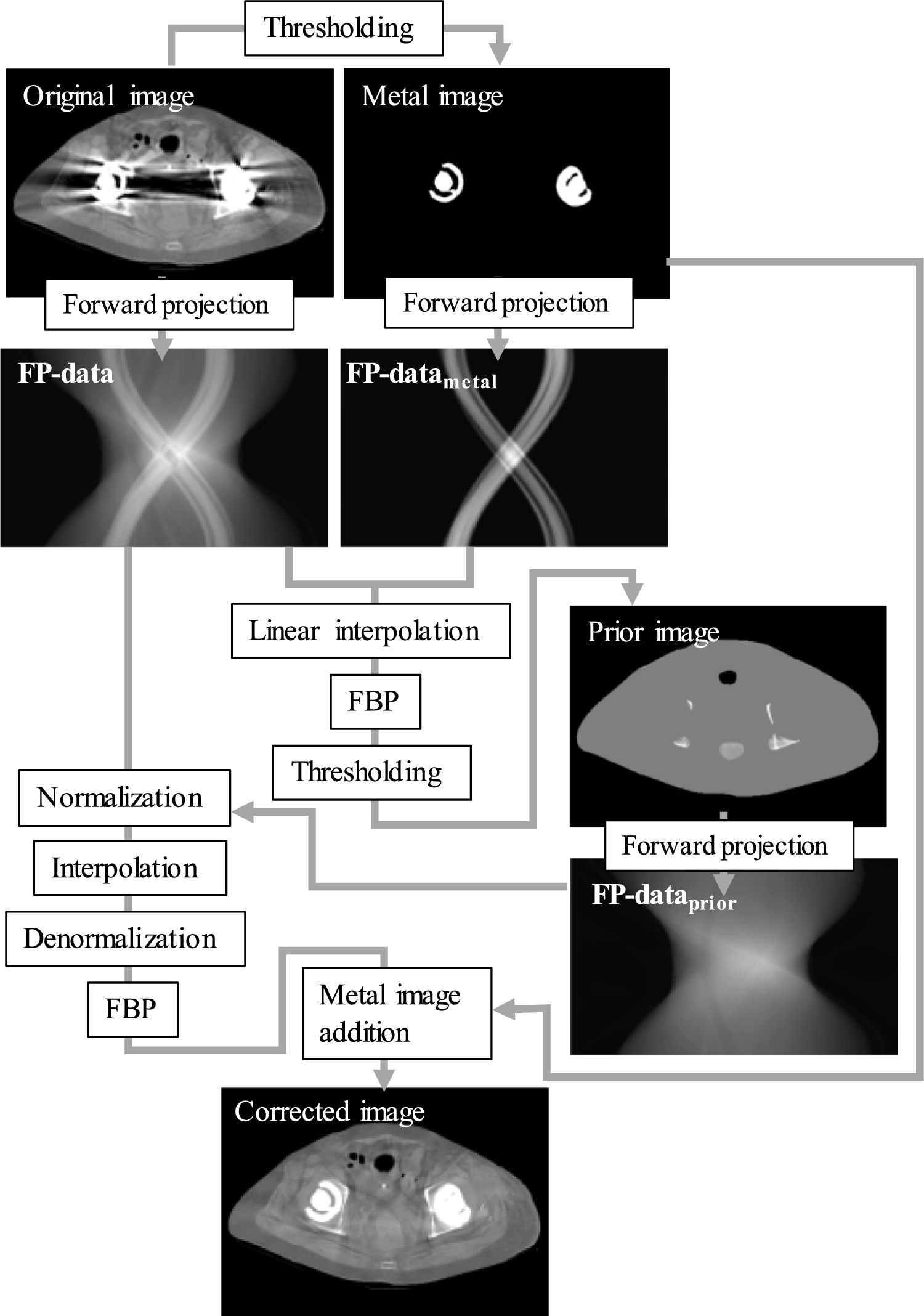
A conventional MAR technique based on projection data normalization (NMARconv) [4] was modified to handle FP-data (FPNMAR). Figure 1 shows an outline of the FPNMAR technique. First, the original CT image with metal artifacts was forward-projected (FP-data). Second, a metal-only image was extracted from the original CT image using simple thresholding; then the image was again forward-projected to produce a projection of the metal trace (FP-datametal). The metal trace was used to identify the regions for inpainting. Third, simple linear interpolation was used to obtain the first MAR image, from which a prior image that had plain and smooth texture was made using thresholding: the air regions were set at − 1000 Hounsfield unit (HU) and the soft tissue parts at 0 HU, while the bone pixels kept their values. The prior image was forward-projected to produce FP-dataprior; then, the FP-data were divided (normalized) by the FP-dataprior and, after linear interpolation, denormalized. Finally, an MAR image was reconstructed from the denormalized projection, followed by an addition of the metal-only image. NMARconv was performed using the original projection data instead of the FP-data and the fan-beam geometry of the CT scanner we used in this study for the forward and back projections.

Outline of the metal artifact reduction (MAR) technique using projection data generated via a forward projection (FP-data). A conventional MAR technique based on projection data normalization (NMARconv) was modified to this version that utilizes FP-data (FPNMAR)

The processing technique used in forward projection was the same as that used in reducing streak artifacts by utilizing FP-data as reported by our laboratory team [3]. The report demonstrated that the CT images reconstructed from filtered FP-data had almost the same spatial resolution as that of the original images and had precisely the same CT numbers. Figure 2 shows the relationship between the coordinates in the FP and those in the rotated CT image data. We employed parallel-beam projection instead of fan-beam projection, which is commonly used in clinical CT systems, because the theory of CT reconstruction assures that fan-beam projection data can be converted to parallel-beam data by a known conversion algorithm [11]. As shown in this figure, we employed a rotation-based method in which a projection data array remains fixed and the image is rotated through interpolation [12]. At each ray position of ri (i = 0, …, N − 1), data sampling at sj (j = 0, …, N − 1) was repeated and accumulated to p(i, k) at each projection angle θk (k = 0, …, n − 1) as follows:

$$p(i,k) = \sum\limits_^ $$

(1)

$$x(i,j) = r_ \cos (\theta_ ) - s_ \sin (\theta_ )$$

(2)

$$y(i,j) = r_ \sin (\theta_ ) + s_ \cos (\theta_ ),$$

(3)

where x and y are the x- and y-sampling positions in the original CT image data c(l, m) (l = 0, …, 511, m = 0, …, 511), respectively, and q(i, j) is the data sampled from c. Bicubic interpolation was used for the sampling with an α parameter of − 0.5 because this method can produce a smaller spatial resolution loss compared with the bilinear technique [13]. The sampling interval was set at half the pixel pitch of the CT image; thus, 1024 points were required (N = 1024) for each of the ri and sj positions. A total of 800 projections (n = 800) were made at intervals of 180°/n within 0° ≤ θ < 180°. This unit of calculation was performed in parallel for i = 0, …, 1023, and k = 0, …, 799 using a GPU capable of highly parallel computing (Geforce RTX4070Ti, Micro-Star Int'l, Taiwan) in combination with a 64-bit central processing unit (CPU) (Core i7-12700, Intel Corporation, California, USA). In this way, the total calculation time was notably reduced. The FP-data in a 1024 × 800 matrix were thus obtained; then, the matrix size was increased to 2048 × 800 by padding zeros on both its left side and right side to enable the filtering process in FBP.

Coordinates in numerical parallel forward projection to generate the FP-data. For each discrete angle θk, along the ray projection at a discrete position ri, sampled data at sj were accumulated to p(i, k). For the sampling, bicubic interpolation was used

Filtering in the FBP was performed using a two-dimensional fast Fourier transform (2D-FFT) function that is incorporated in the development environment for the GPU (Compute Unified Device Architecture: CUDA, Nvidia). This function is optimized for the architecture of the GPU and can perform a 2D-FFT for a 2048 × 800 matrix in less than 1 ms. After the filtering, a back projection process was performed as follows. For each pixel location of x′(l, m) and y′(l, m) in an image to be reconstructed, the r position rl, m in the filtered projection data at θk can be calculated as follows:

$$r_ = x^(l,m)\cos (\theta_ ) + y^(l,m)\sin (\theta_ ).$$

(4)

The sampling data τ (l, m, k) at r in the projection data at θk were obtained through one-dimensional cubic interpolation with an α parameter of − 0.5; then the sampled data were integrated (back-projected) to the pixel c′ (l, m) as follows:

$$c^(l,m) = \sum\limits_^ .$$

(5)

These calculations were parallelized for l = 0, …, 511, and m = 0, …, 511 using the GPU.

The display field of view (DFOV) varies depending on the diagnostic purposes. As a result, there is some capriciousness with FP-data, which affects its performance in MAR. Since metal artifacts frequently spread to areas outside the object, CT number alterations due to spread artifacts are generally ignored when the DFOV includes only the object’s contour. Moreover, when the DFOV is set in a size smaller than the contour, the CT number alterations are further ignored. Naturally, metal artifacts caused by metals outside the DFOV cannot be compensated for; thus, such artifacts are not covered by FPNMAR. While being aware of these problems, we performed the FPNMAR and evaluated its MAR performance.

Images of hip prostheses, dental fillings, and coils in brain aneurism coiling in clinical cases scanned with a 64-slice CT scanner (Somatom Definition Edge, Siemens Healthineer, Germany) were processed by the FPNMAR. Two clinical cases each of hip prosthesis and dental filling were selected for a comparison between FPNMAR and NMARconv. These cases are the same ones used in a previous study of our laboratory team [14] that purposed improvement of image texture in the MAR image generated using original projection data. To quantitatively compare the artifact strengths of the two NMAR methods, we measured the normalized artifact index AIn, which is defined as follows:

$$ \ }}_}}=\frac}}_}}}^-}}_}}}^}}}}_}}},$$

(7)

where SDA denotes the standard deviation (SD) measured of the CT image with metal artifacts; SDB is the SD measured of the CT image with no metal artifacts [15]. The normalization using SDB was adopted because the spatial resolution of the image reconstructed based on the FP-data is slightly different from that of the image reconstructed from the original projection data. The region of interest (ROI) with 20 × 20 pixels for SDA was placed at a central position between both hip joints in the bladder for the hip prosthesis case and the lingua for the dental filling cases. The ROI for SDB was placed in the soft tissue with no visible structures in muscles around the ilium or the oropharynx. Thus, for each case, a single SDB was obtained by averaging the SD values of the ten selected images and was used as the common value for SDB for AIn calculations of the ten consecutive images with metal artifacts. The AIn values were compared between FPNMAR and NMARconv, by means of the Wilcoxon signed-rank test with p < 0.05 taken as statistically significant.

This retrospective use of the image and projection data was approved by our institutional review board, and since we performed only additional image reconstruction, the requirement for written informed consent was waived for all the patients.

For FP-data generation, FP-data filtering, back projection, and the total processing in FPNMAR, the computation time was measured for ten CT images selected from those used in this study. For comparison between with and without the GPU, we rewrote the FPNMAR program using normal sequential codes and then measured computation time. The filtering of FP-data was performed using a 2D-FFT function provided in Intel Math Kernel Library 2019. The built-in timer in the Microsoft visual C++ 2013 was used for the measurement.