1 Introduction

A fundamental aspect of motor vehicle driving, and locomotion in general, is to find an adequate balance between progress and caution. The main purpose of driving is typically to get to the destination as efficiently as possible. However, one also needs to make sure to get there without crashing and avoid other undesired consequences such as getting ticketed. A key challenge here is to manage the uncertainty inherent in most traffic situations. For example, will the vehicle in front brake and, if so, how hard? Is there a risk of a pedestrian suddenly appearing behind the stopped bus ahead? Being too pessimistic about how a traffic situation may play out in uncertain situations could lead to overcautious behavior or even a complete lack of progress. Moreover, non-human-like, overcautious, behavior may be surprising to other road users with potential negative safety consequences (Dinparastdjadid et al., 2023). Yet, being too assertive in an uncertain situation may incur a significant risk of collision.

Human drivers are most often able to manage this tradeoff, even in highly complex and uncertain traffic situations. Thus, understanding how human drivers manage uncertainty is critical for developing realistic and explainable computational models of their behavior. Such models have a range of applications such as explaining crash causation (Summala, 1996), representing other road users in traffic simulation (Treiber and Kesting, 2013; Igl et al., 2018; Suo et al., 2021; Markkula et al., 2023), establishing behavior benchmarks for autonomous vehicles (Engström et al., 2024), or as part of the AV software itself (Sadigh et al., 2018).

Contemporary generative AI models can learn complex driving behaviors from large quantities of data (e.g., Suo et al., 2021; Igl et al., 2022). There has also been extensive work in machine learning and robotics on developing models able to manage uncertainty through concepts like artificial curiosity and intrinsic motivation (e.g., Schmidhuber, 1991; Sun et al., 2011; Hester and Stone, 2012). However, due to the black-box nature of these models, they do not lend themselves to explaining the cognitive mechanisms underlying human adaptive behavior, which is also typically not their purpose.

There is a long-standing tradition in traffic psychology in modeling adaptive road user behavior, such as the regulation of speed and headway. Models in this tradition, often referred to as motivational models, include the risk homeostasis theory (Wilde, 1982), the zero-risk theory (Näätänen and Summala, 1976; Summala, 1988), and the task capability interface (TCI) model (Fuller, 2005) (see Lewis-Evans, 2012 for a review). In these models, excitatory “forces” such as the motivation to make progress toward the destination are balanced against inhibitory “forces” where uncertainty is typically a key component. However, these traditional motivational driving models are typically conceptual in nature, lacking mathematical rigor.

One example of an early computational model of adaptive driving behavior, of particular relevance for this paper, is the pioneering work by Senders (1967) based on the visual occlusion paradigm. In visual occlusion, subjects wear a helmet featuring a visor that, while driving, intermittently occludes the subject's view. The occlusion and viewing times may be fixed, or the subject could be given control over the occlusion time by means of a switch that opens the visor for fixed viewing time period (typically 0.25–1 s). Senders et al. found that, when occlusion times were controlled at different levels, subjects adapted their speed such that shorter occlusion times resulted in higher speed and vice versa. Conversely, when subjects had voluntary control over the occlusion time, and speed was controlled, higher speeds led to shorter occlusion times and vice versa. To explain these results, the authors developed an information theoretic model based on the idea that uncertainty builds up during the occlusion intervals and that the observed adaptive behaviors (speed and occlusion interval adjustments) reflects the attempt of the driver to control this uncertainty. Senders et al. further proposed two main sources of uncertainty in driving that need to be controlled: (1) the uncertainty about the traffic situation ahead due to loss of relevant visual information and (2) uncertainty about the vehicle's position on the road due to random disturbances in vehicle lateral control.

These early occlusion results have since been replicated for other types of driving scenarios. For example, in a recent study, Pekkanen et al. (2017) found reduced voluntary occlusion times with reduced headway. Pekkanen et al. (2018) developed a computational model of drivers' visual sampling where uncertainty about the consequences of action (acceleration), resulting from uncertainty in state estimation, was used to directly control attention (operationalized as a voluntary opening of the occlusion visor).

Victor et al. (2005) analyzed drivers' visual time-sharing between driving and a secondary task and found, in line with the occlusion studies, that the visual demand of driving during curve negotiation led to reduced off-road glance durations. Johnson et al. (2014), based on earlier computational modeling in non-driving domains (Sprague and Ballard, 2003), proposed a model of visual time-sharing during car following based on a tradeoff between task priority and uncertainty.

Most computational models of human adaptive driving behavior have focused on visual sampling and models with a more general behavioral scope are rare. One notable exception is the model by Kolekar et al. (2020), based on zero-risk theory and the field of safe travel concept from Gibson and Crooks (1938). The model represents uncertainty about potential collisions in terms of a dynamical risk field, and was demonstrated to account for a wide range of empirical adaptive driving behavior results reported in the literature. However, the current version of the model is limited to static scenarios with no other road users present.

Another example of a generic computational model of adaptive behavior, related in some ways to Kolekar et al.'s (2020) field model, is the model developed by da Lio et al. (2023) based on the affordance competition hypothesis originiating in neuroscience (Cisek, 2007). The concept of affordances were introduced by Gibson (2014), based on the earlier field of safe travel model (Gibson and Crooks, 1938). Affordances refer to opportunities for action offered to an agent by its environment. For example, a chair affords sitting and an empty adjacent lane affords overtaking the car ahead. The model by da Lio et al. implements a control architecture with a set of affordances (e.g., stay in the current lane or move to the next lane) which compete for action control, where the selection of affordances is based on a reward function which can be set to represent desired driving characteristics (e.g., avoid collisions, follow the road rules etc.). It was demonstrated that a wide range of relative complex human-like driving behaviors emerges from this general architecture, such as merging onto a highway, overtaking a lead vehicle, responding to a cut-in event and interacting with a pedestrian at a crosswalk. The affordance concept has also been used as a basis for action-based representations in machine learning-based driver models (e.g., Xiao et al., 2021).

A common denominator in most of these existing models is that adaptive driving behavior is, on the one hand, driven by a motivation to achieve goals and, on the other, by inhibitory motives such as the need to control uncertainty. The computational models reviewed above typically represent specific aspects of this phenomenon (e.g., visual sampling and time-sharing), except for a few notable developments of models with a more general scope (Kolekar et al., 2020; da Lio et al., 2023). However, a generic computational model of adaptive driving behavior, applicable across all types of scenarios and behaviors, is still lacking.

In this paper, we propose such a model based on active inference, a behavior modeling framework originating from computational neuroscience (Friston et al., 2017; Parr and Friston, 2017; Parr et al., 2022). The application of active inference, and the closely related predictive processing framework (Clark, 2013, 2015, 2023), in the automotive domain were explored in Engström et al. (2018), but only conceptually. In a series of recent papers (Wei et al., 2022, 2023a,b), we have demonstrated how computational driver models based on active inference can be implemented and learned from data, thus offering a potential “middle ground” between traditional “black box” machine learning models and mechanistic human behavior models. In this paper, we focus specifically on how active inference can provide a conceptual and computational basis for modeling human adaptive driving behavior and, in particular, how a (Bayes) optimal balance between goal-directed action and the resolution of uncertainty emerges “automatically” from the minimization of expected free energy.

In active inference, the agent estimates the free energy associated with alternative future policies, π, defined as sequences of actions π = a1:H within a predefined planning time horizon H, and, at each time step, selects the action associated with the policy that has the lowest expected free energy (EFE). Expected free energy can be formulated in several different ways (see Friston et al., 2015, 2017; Parr et al., 2022. For present purposes we choose the formulation in Equation (1) which defines the expected free energy as the (negative) sum of a pragmatic value and an epistemic value, where the pragmatic value relates to goal seeking behavior and epistemic value to information-seeking (uncertainty-resolving) behavior, mapping conceptually to progress vs. caution or exploitation vs. exploration.

EFE=G(π)=-?Q(o|π)[logP(o)]︸Pragmatic value-?Q(s,o|π)DKL[Q(s|o,π)||Q(s|π)]︸Epistemic value    (1)

In Equation (1), s = s1:H and o = o1:H are sequences of future states and observations within the lookahead time horizon H, E denotes expectations, and DKL denotes the Kulback-Leibler (KL) divergence, a statistical measure of the distance between two distributions. Q(o|π) and Q(o, s|π) are the agent's belief or prediction about future observation and state-observation sequences, respectively.

In the formulation of expected free energy in Equation (1), the pragmatic value is defined based on a prior probability distribution over observations P(o) that is biased such that observations preferred by the agent have the highest probability and, hence, the highest pragmatic value. Thus, selecting policies that generate preferred observations will maximize the pragmatic value and contribute to minimizing the expected free energy. This hence implements a mechanism that generates goal-directed (or aversive) behavior, in a similar way as optimizing against a reward or cost function in optimal control or reinforcement learning (Sutton and Barto, 2018).

The epistemic value represents the value of obtaining new information that may help to resolve uncertainty in the belief about future states. This may, in turn, enable (or “open up”) new policies that maximize pragmatic value and thus realize the agent's preferred observations. For example, when planning to overtake a car ahead, there is typically uncertainty about whether this will lead to a conflict with a potential vehicle approaching from behind in the adjacent lane. The uncertainty can be resolved by checking the rearview mirror to verify that the lane is clear. Epistemic value scores such information-seeking actions, contributing to the overall expected free energy. In Equation (1), the epistemic value of a policy is defined as the expected KL divergence between the agent's prior belief Q(s|π) and posterior belief Q(s|o, π) about external states associated with that policy, corresponding to (expected) Bayesian Surprise (Itti and Baldi, 2009; Dinparastdjadid et al., 2023). Intuitively, this means that epistemic value is maximized for observations that lead to a maximum change in beliefs. Epistemic value can also be expressed as in Equation (2), as the difference between the posterior predictive entropy and the expected ambiguity (Parr et al., 2022, p. 135):

?Q(o|π)DKL[Q(s|o,π)||Q(s|π)]=H[Q(o|π)]-?Q(s|π)H[P(o|s)]    (2)

where H denotes Shannon entropy.

In Equation (2), the posterior predictive entropy (first term; H[Q(o|π)]) represents the uncertainty about future observations associated with a given policy. That is, a policy with a high posterior predictive entropy may yield a variety of different observations with a strong potential for gaining new information. The expected ambiguity (second term; ?Q(s|π)H[P(o|s)]) represents the expected diversity of observations for a given state. Intuitively, this means that the epistemic value of a policy is discounted if the state to be visited does not generate reliable observations (e.g., due to darkness or otherwise reduced visibility). Thus, epistemic value is maximized when the expected ambiguity is zero, that is, when the observation generated by the policy is expected to completely resolve the uncertainty.

Thus, in uncertain situations, minimizing expected free energy “automatically” promotes policies with high epistemic value, generating observations expected to resolve the uncertainty. As we will see below, a single action (e.g., moving forward) often carries both pragmatic (moving closer to the goal or away from danger) and epistemic value (getting a better view to resolve uncertainty). This leads to a key distinguishing feature of active inference: Goal directed (pragmatic) and information-seeking (epistemic) value are defined in a common currency and an optimal balance between them (given the agent's beliefs and preferences) can be established by minimizing the expected free energy.

The key objective of this paper is to demonstrate how active inference can provide a novel conceptual and computational basis for modeling adaptive driving behavior. We explore how uncertainty can be resolved “on the fly” as an integral part of the general planning objective to minimize expected free energy. Specifically, we demonstrate how a model based on the single mandate to minimize expected free energy can account for two apparently disparate adaptive driving behaviors: (1) safely passing an occluding object and (2) visual time-sharing behavior, for example when texting on a cell phone.

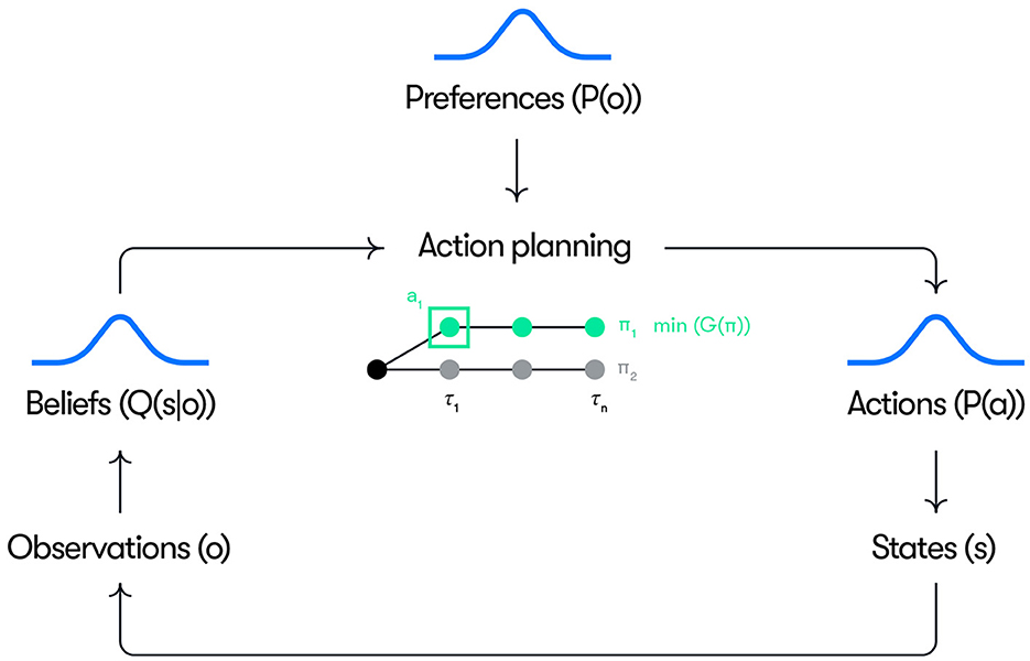
2 Materials and methods 2.1 Overview

A conceptual overview of our model is given in Figure 1. Control actions (e.g., acceleration and steering inputs) are generated as the result of a planning process where policies π, constituting sequences of future actions up to the planning horizon, are selected based on identifying the policy with the minimum expected free energy (i.e., minπG(π)). At each time step, the first action of the selected policy is executed. The action planning is based on the driver's beliefs over hidden states Q(s) and preferences defined as priors over observations P(o). The beliefs are continuously updated into posterior beliefs Q(s|o) based on new observations. The precision (inverse variance) of the beliefs represents the certainty of these beliefs over states. The preferences P(o) define the observations that the driver is seeking to realize through action (e.g., maintain a speed near the speed limit) and their precision represents the “strength”, or priority, of the preference (i.e., how motivated the driver is to keep the speed near the speed limit).

Figure 1. Schematic overview of the model. See the text for explanation.

In action planning, a set of alternative counterfactual policies are sampled at each time step t and rolled out up to a time horizon representing the planning window. In all simulations reported here, a planning horizon of 4 s is used. For each candidate policy, the beliefs over states are propagated forward in time from the current belief based on a state transition model and the propagated beliefs are used to calculate the counterfactual pragmatic and epistemic value at each future time step, τ, in the planning window. The prior preferences are used to score the pragmatic value based on the counterfactual observations generated, where the pragmatic value at a given future time step, τ, is computed based on the probability of the counterfactual observation made at that time step under the preference distribution. Similarly, epistemic value is computed based on counterfactual beliefs about future states and observations. The overall expected free energy of each policy is then scored based on Equation (1) and (2) (as the negative sum of the epistemic and pragmatic values over the planning horizon), and the action at the next time step is sampled from a distribution of the first actions in the highest scoring policies. These general principles can be implemented in many different ways, where the current implementation is based on a particle filter, as described in more detail below.

The driver's generative model is represented as a discrete-time Partially Observable Markov Decision Process (POMDP) which describes how hidden environment states (e.g., pose of the ego vehicle) evolve over time depending on the ego vehicle driver's chosen policies and resulting control actions, and generate signals observed by the driver, for example the new pose of the ego vehicle or the presence of a pedestrian. Importantly, some of these state variables are not always directly observable to the driver, for example, the driver cannot observe a pedestrian when they are occluded by an object and cannot observe the road ahead while looking away from the road.

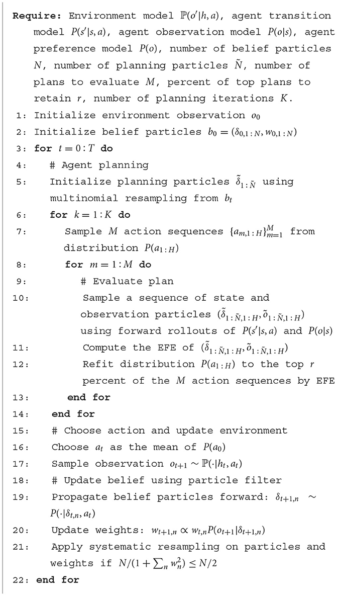
The model uses a mixture of discrete and continuous state, observation, and action variables with highly structured dependencies, which makes exact computation of the belief update and action selection intractable. We thus perform approximate belief update and policy/action selection using a particle filter and a particle planner. At a high level, this means that the model represents uncertainty about the hidden states using an ensemble of hypothetical states, where each ensemble member represents a different possibility. The model then selects the best actions by simulating future state-action-observation trajectories under different policies using a state transition model and an observation model and scores each policy for expected free energy using Equation (1) and (2). Such a simulation-based inference method is known to approach the theoretically optimal (or exact) solution with a large number of particles (Murphy, 2012).

2.2 Implementation

In this section, we first describe the perception and action process of active inference agents. We then describe our particle-based implementation.

2.2.1 Active inference and expected free energy

We use the standard notation for POMDP (Kaelbling et al., 1998), where S = denotes a set of states, A = denotes a set of actions, O = denotes a set of observations. The active inference agent has a generative model of the environment which consists of a state transition distribution P(s′|s, a) and an observation distribution P(o|s). We denote the environment (also known as the generative process in the active inference literature; Parr et al., 2022) that the agent interacts with as ℙ(o′|h, a), where the time-indexed ht = (o1:t, a1:t−1) is the interaction history.

Upon receiving an observation ot ~ ℙ(·|ht−1, at−1) from the environment, the agent updates its belief, defined as a probability distribution over the hidden environment state Q(st), by minimizing the variational free energy of its generative model (see Parr et al., 2022). The optimal belief distribution is known to have the form given by Equation 5 (Da Costa et al., 2020):

Q(st)∝exp(logP(ot|st)+?Q(st-1)[logP(st|st-1,at-1)])    (3)

Starting from the updated belief, the agent constructs predictions over future state-observation trajectories (st+1:t+H, ot+1:t+H) for a lookahead horizon of H time steps given a policy π = at:t+H−1. These predictions, defined over the lookahead time steps τ∈ in the form of probability distributions, can be constructed sequentially (i.e., via rollout) as follow:

Q(oτ,sτ|π)=?Q(sτ-1|π)[P(oτ|sτ)P(sτ|sτ-1,aτ-1)]    (4)

The quality of each policy is scored by the expected free energy function defined in Equation (1) as:

G(π)=∑τ=t+1t+H−?Q(oτ|π)[logP(oτ)]︸Pragmatic value−?Q(sτ,oτ|π)DKL[Q(sτ|oτ,π)||Q(sτ|π)]︸Epistemic value 2.2.2 Particle-based algorithm

We use a particle-based approach to belief representation, inference, evaluation, and planning. We describe these components below and summarize the entire process as pseudocode in Algorithm 1.

Algorithm 1. Simulation of particle-based active inference agent.

Using a particle filter, we represent the ego's belief bt over all state variables using a set of N particles ,δn∈R|S|, where each particle consists of a vector corresponding to a realization of the state variables and a weight wn≥0,∑nwn=1 representing the likeliness of the realization under the ego's belief distribution. Under this representation, the ego belief has high certainty (high precision) if all particles with high weights are similar, for example, all particles correspond to the pedestrian being present, and low certainty if all particles have even weights and are substantially different, for example, the element representing the pedestrian's position in each particle is evenly distributed on the road map.

Upon executing an action at and receiving a new observation ot+1, we update the set of particles, including both the state vectors and weights, using a Sequential Importance Resampling (SIR) filter (Murphy, 2012). The SIR filter first samples a next state conditioned on the current state and action and updates the weights using Equation 5:

wt+1,n∝wt,nP(ot+1|δt+1,n)    (5)

where δt+1, n~P(·|δt, n, at).

To address the mode collapse problem common in particle filters, we use a large number of samples and apply systematic resampling so that the sampled particle weights are equidistant. Resampling of the current set of particles is only performed if the effective sample size Neff≈N/(1+∑nwn2) is less than N/2. In this way, low weight particles are still represented.

2.2.3 EFE computation

Evaluating the EFE of an action sequence under a particular belief requires propagating the belief particles to compute the state and observation distributions at each counterfactual future time step and using the propagated particles to evaluate the pragmatic and epistemic values.

The particles can be easily propagated by recursively sampling the next state from the transition distribution conditioned on the previous sampled state and policy action and then sampling the next observation from the observation distribution conditioned on the sampled next state, i.e., Equation (4). To evaluate the pragmatic value [the first term in Equation (1)], we compute the average log likelihood of each observation sample under the preference distribution.

To compute the epistemic value [term 2 in Equation (1)], we use the decomposition of the expected information gain in Equation (2), which is the difference between the posterior predictive entropy and the expected ambiguity:

?Q(o|π)DKL[Q(s|o,π)||Q(s|π)]=H[Q(o|π)]-?Q(s|π)H[P(o|s)]

We approximate the intractable posterior predictive entropy using a Kernel Density Estimator [similar to Fischer and Tas (2020)].

2.2.4 Model predictive control

Given each updated belief, we compute the approximately optimal EFE-minimizing actions using the Cross Entropy Method (CEM) for model predictive control (De Boer et al., 2005). CEM iteratively refines a distribution over action sequences (i.e., policies) by sampling a batch of action sequences, simulating their trajectories forward, selecting the top r percent scoring trajectories, and refitting the action distribution to the selected action sequences. This process can be understood as sampling from a distribution of action sequences in proportion to their EFE values similar to relative entropy policy search (Peters et al., 2010).

Our application of CEM has two major differences from its normal use in optimal control and trajectory optimization. First, the optimal decision for an active inference agent is based on its belief as opposed to a known state. Thus, we adapt the default CEM by treating a set of belief particles as the state. Specifically, we draw Ñ particles from the belief set according to their weights as the input to the CEM planner. This allows us to compute EFE using sampled-based averaging during policy search. Second, we use a mixture of discrete (e.g., gaze direction) and continuous actions (e.g., vehicle control) in the visual time-sharing scenario, whereas the default CEM typically only optimizes continuous actions. We solve this by separately fitting the discrete and continuous variables once the best trajectory samples are selected in each iteration.

3 Results

This section describes the simulation results from applying our model to two different driving scenarios that require the control of uncertainty: (1) passing an occluding object and (2) visually time-sharing gaze between driving and a secondary task. In the first scenario, the uncertainty concerns the potential presence of a pedestrian hidden behind the object who may step into the ego vehicle's path. In the second scenario, uncertainty about the lateral position of the vehicle in the lane builds up during glances away from the road due to disturbances such as wind gusts and an uneven road surface (Senders, 1967).

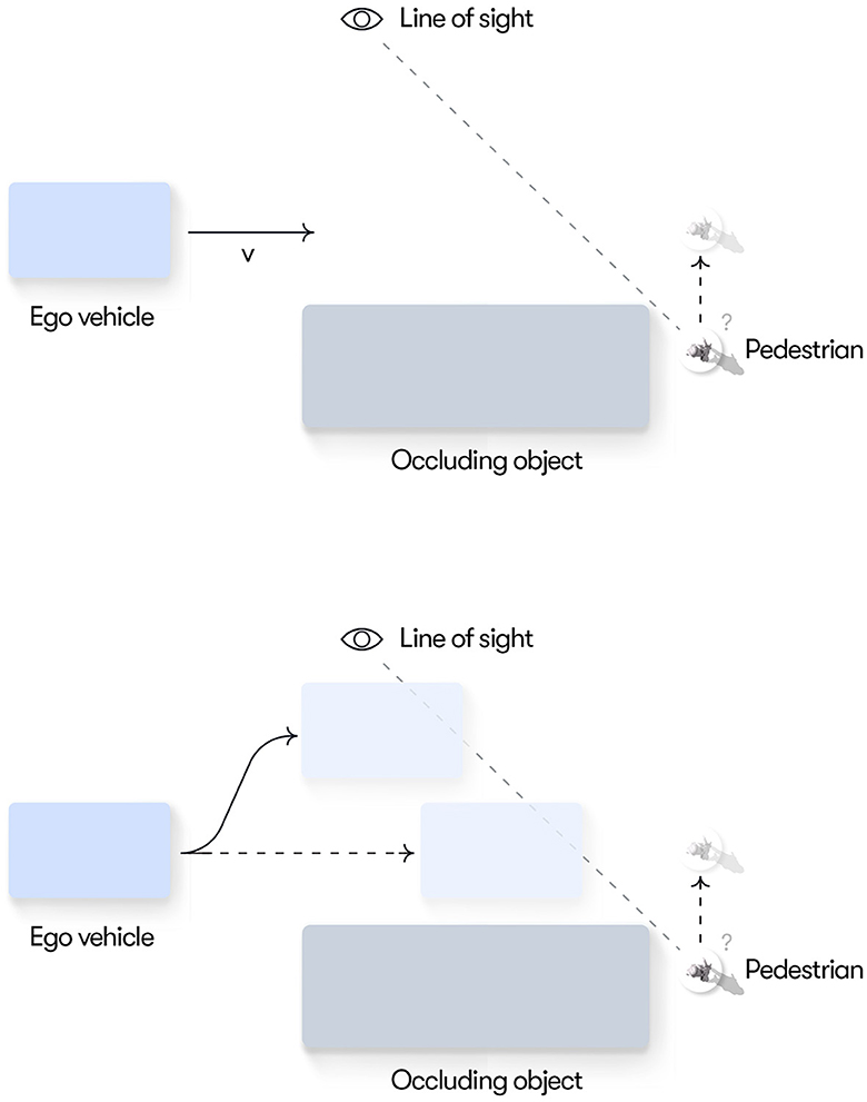
3.1 Scenario 1: passing an occluding object

In this scenario, the ego vehicle approaches a large occluding object (e.g., a stopped bus) and there is uncertainty about whether a pedestrian, potentially hidden behind the object, will encroach into the ego vehicle's path (see Figure 2). Managing uncertainties around occlusions is a key behavior that must be mastered both by human drivers and autonomous vehicles and thus an interesting first use case for our model. We make the simplifying assumptions that a single pedestrian is the only possible obstacle that could be hidden behind the object and that, if a pedestrian is present, it will always step out in the road and cause a potential conflict with the ego vehicle. We further assume that the pedestrian can only be present at a given point along the horizontal (x) dimension so that it, if present, always becomes visible when it gets into the line of sight of the ego vehicle driver (see Figure 2). These assumptions simplify the current model implementation but they do not impose any fundamental limitations on the general modeling framework.

Figure 2. Conceptual illustration of Scenario 1. (Top) The ego vehicle driver ideally wants to keep speed as close as possible to the speed limit. However, until reaching the line of sight, the driver is uncertain whether a pedestrian is hidden behind the double-parked vehicle and thus needs to adapt their speed to make sure they can stop short of the location where a pedestrian may appear. (Bottom) By moving left, the ego driver could reach the line of sight earlier, thus resolving the uncertainty sooner and potentially enabling more efficient passing of the occluding object.

We further assume that, as a default, the ego vehicle driver prefers to keep the speed at the speed limit to maximize progress while respecting the rules of the road. However, if the driver believes that there is a risk for a hidden pedestrian encroaching into their path, they need to adapt their speed to be able to stop well ahead of the pedestrian (to meet the preference of conflict avoidance) without harsh braking (to meet their preferences for deceleration comfort). When the ego vehicle reaches the line of sight, the driver's uncertainty about the presence of the pedestrian is resolved and, if no pedestrian is present, they can speed up again to the preferred speed. Furthermore, as shown in Figure 2, bottom, by moving left in its lane the ego driver can reach the line of sight earlier, thus resolving the uncertainty that hinders progress and enabling a potentially faster trajectory past the occluding object. The general goal of the current simulation is to demonstrate how these adaptive driving behaviors emerge solely on the basis of minimizing expected free energy.

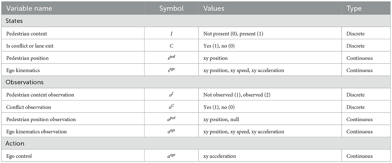
3.1.1 Model specification

The state, observation and action variables in the model are listed in Table 1. The ego vehicle kinematic states are denoted as sego=[x,vx,ax,y,vy,ay] and are assumed to follow linear dynamics. In this scenario, we model the ego vehicle simply as a point mass which was motivated by the desire to keep the model as simple as possible. Since the source of uncertainty here is the presence or absence of the pedestrian, a point mass dynamics model is sufficient to illustrate the key model principles of interest. By contrast, in Scenario 2, where the main source of uncertainty is the vehicle position on the road, we replaced the point mass model with a bicycle model, as further described below. The pedestrian's position sped = [x, y] is determined by a context variable, I, denoting whether the pedestrian is present or not present. If the pedestrian is present, its x and y positions will be set next to the occluding object. Otherwise, its x and y position will be set to a null value far away from the ego vehicle (e.g., −1,000). C represents whether there is a conflict between the ego and the pedestrian or if the vehicle exits the lane, in which case C is set to 1, and 0 otherwise. A conflict is defined as the pedestrian being present and the longitudinal distance between the ego and the pedestrian is less than a safe distance (2 m).

Table 1. State, observation and action variables in the POMDP for Scenario 1.

As described above, the main source of uncertainty in this scenario is that the presence or absence of the pedestrian cannot be determined before the vehicle reaches the line of sight. Geometrically, as shown in Figure 2, the pedestrian is occluded if it is behind (i.e, with smaller x coordinate) the line of sight connecting the ego vehicle and the upper right tip of the occluding object (since we are modeling the ego vehicle as a point mass, this is also the reference point from which the observation is made). For the observation space, we introduce a variable oI to represent the context observed by the ego. oI is set to “observed” when the ego vehicle enters the line of sight, otherwise, it is set to “not observed”. The rest of the observation variables share the same semantics and dimensionality as the underlying state variables, except when the pedestrian is occluded. In this case, the observations of the pedestrian's position, oped, are set to null. Hence, as long as there is no occlusion, we assume no uncertainty over the observations and that, hence, the ego can observe both its own and the pedestrian's kinematics states exactly.

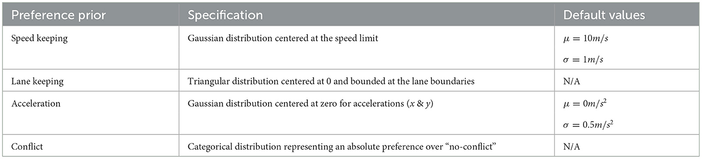
As described above, the model's preferences are defined as priors over observations. The preferences of the model used in Scenario 1 and their default values are given in Table 2. The default parameter values were set by hand and no systematic model optimization was performed. Again, the key purpose was to demonstrate the basic model principles rather than to achieve optimal performance. All simulations were run with a 200 ms time step (i.e, an update frequency of 5 Hz). Due to the stochasticity of the model, each simulation run yields a unique trace. However, for clarity, we only plot randomly selected single simulation traces.

Table 2. Preference priors for Scenario 1.

3.1.2 Simulations

This section presents the results of different permutations of the occlusion scenario with the purpose to illustrate the key aspects of our model described above. We begin with the case where the ego driver can only drive straight (i.e., not move laterally, e.g., due to a narrow lane) and then extend this to allow for lateral movement that enables the driver to resolve uncertainty earlier through epistemic action (moving left to reach the line of sight earlier). In all simulations, we assume that no pedestrian is actually present while the ego driver model may, or may not, initially believe that a pedestrian could be present with a given probability.

3.1.2.1 Simulation 1a: safely passing an occluding object

The purpose of this initial simulation is to show how our active inference model generates successful adaptive behavior in the occlusion scenario, finding an optimal balance between progress and caution given its set beliefs and preferences. Since, in this first simulation, the driver can only drive straight and not move laterally, the ego driver's preferences reduce to prior d