Individuals with SCD or MCI were included from the Swedish BioFINDER-1 study (clinical trial no. NCT01208675). The study protocol is described in detail before [27]. Briefly, the consecutively recruited participants in BioFINDER-1 are aged between 60 and 80 years, perform ≥ 24 points on the MMSE, and have been referred to any of the participating memory clinics due to cognitive complaints. A neuropsychological assessment including a comprehensive test battery was used to classify participants as SCD or MCI as previously described [28]. All patients with MCI were classified based on the DSM-5 criteria for MCI [29]. Note however, that for this study the SCD and MCI groups were analyzed together, since the aim of the project was to develop methods that would be useful for longitudinal predictions in an unselected group of patients with cognitive complaints, prior to dementia. Exclusion criteria were cognitive impairment that could be better accounted for by another non-neurodegenerative condition, severe somatic disease, and current alcohol or substance abuse. Only patients with available baseline MRI scans and longitudinal cognitive follow-up of at least four years from baseline were included here. Demographic information (age, sex, education), APOE ε4 carriership status (negative/positive) and baseline cognition (MMSE score and Alzheimer’s Disease Assessment Scale [ADAS] delayed word recall) were collected for all individuals.

To guarantee reproducibility and robustness of the models, a double cross-validation scheme was used, such that the data from all individuals could be utilized for both training, validation and test. A five-fold division into development set (80%, used for training and validation) and test set (20%) was used. A stratified random split was used, such that there was no significant difference between development and test sets in the distribution of diagnosis, age, education, sex, or APOE status. The stratified random split was produced by randomly splitting the dataset until a division fulfilling the constraints was obtained. For the development sets a 10-fold cross-validation was used, where the folds were drawn such that the same ratio of early AD and non-AD was obtained for each fold, but otherwise randomly. Similarly to the division into test and development, the stratified random split was produced by randomly splitting the dataset until a division fulfilling the constraints was obtained. The double cross-validation scheme was chosen to get robustness and good estimates of the uncertainties of the results. An overview of the demographics for the cohort can be seen in Table 1.

A sub cohort of the Alzheimer’s Disease Neuroimaging Initiative (ADNI) dataset was used for independent evaluation. All participants included had MCI at baseline, at least four-year longitudinal cognitive follow-up from baseline and either MCI or AD dementia after four years. The same variables as included from the BioFINDER cohort where included, including MRI images. An overview of the demographics for the cohort can be seen in Table 1.

There were two outcomes of interest. The primary binary outcome was four-year progression to AD dementia, where a clinical diagnosis of AD dementia during the four years follow-up was considered as a progression. Clinical status of AD dementia was evaluated according to the DSM-5 criteria for major neurocognitive disorders and recorded at each visit by a senior neuropsychologist and experienced memory disorder specialist. Additionally, a diagnosis of AD dementia was only used if the participant had an abnormal cerebrospinal fluid profile consistent with AD pathological change. The diagnostic process is described in detail in [27]. The primary continuous outcome was four-year cognitive decline as measured by the change from baseline in the MMSE score. MMSE is a measure of global cognition, and ranges from 0 to 30 where lower scores indicate worse cognition. Four-year cognitive decline was measured by fitting linear regression models for each individual separately using all available follow-up data within four years from baseline, then extracting the estimated regression slope.

T1-weighted MRI was performed on a 3T Skyra MRI scanner (Siemens Healthineers, Erlangen, Germany) producing a high-resolution anatomical MP-RAGE image (TR = 1950 ms, TE = 3.4 ms, 1 mm isotropic voxels, 178 slices). The MRI images were minimally processed using skull stripping, bias correction, and normalization to MNI152 template space [30] using ANTS [31] (normalized using a multi-resolution level [shrink factors = 8, 4, 2, 1, and smoothing sigmas = 3, 2, 1, 0] approach with rigid [mutual information metric 32 bins, regular sampling 25%], affine [mutual information metric 32 bins, regular sampling 25%] and SyN [affine + deformable, cross correlation metric, search radius = 4, full sampling]). Cortical reconstruction and volumetric segmentation were performed with the FreeSurfer image analysis pipeline, as described previously [32]. The Jacobian determinant (JD) images where computed based on the anatomical MRIs non-linear warp to template space and quantify the local deformations, wherein reduced brain matter and atrophy are gauged. Thus, the MRI images are used in native space, as a normalization to MNI space could erase the crucial information, while the JD images are in MNI template space as they map out the expansion/contraction of voxels relative a normal brain and are expected to add some information to the MRI in the form of tissue loss and atrophy relative a normal template brain.

Several a priori measurements are related to change in cognition, wherefor we investigated several different types of data and models, see Fig. 1. The first model [“Clinical data model”] utilized readily available demographics information (age, sex, and education), MMSE score, ADAS delayed word recall [33] and APOE status. The second model [“Hippocampal volume model”], used hippocampal volume (average of left and right hemisphere) as well as intracranial volume added to the clinical data model. The third model [“FreeSurfer model”], used regional brain volumes from the FreeSurfer pipeline together with intracranial volume added to the clinical data model. The fourth model [“DL model”] used whole brain MRI and JD images along with the clinical data variables in a CNN model. The different models are described in more detail below.

Overview of study. The study consisted of three parts: participant selection, model fitting, and model evaluation

For the clinical data model and the hippocampal volume model we trained logistic regression models for prediction of progression to AD dementia and linear regression models for prediction of longitudinal cognitive decline. For the FreeSurfer models, random forest was used.

For all of the models the features were standardized by removing the mean and scaling to unit variance. The models were optimized using the Scikit-learn library (v. 0.22) in Python (v. 3.5) [34]. For the random forest models, the random forest classifier was used for prediction of progression to AD dementia and the random forest regressor was used for prediction of longitudinal cognitive decline, both with default parameters.

CNNs work by learning a successively more complex representation of images across its increasing layers, where the earliest layers closest to the input image are activated by simple shapes such as edges, followed by more complex structures. This method of creating an increasing complex visual representation is similar to how the brain’s visual cortex processes images. We used the CNN architecture suggested by Spasov et al. [14], which is a parameter-efficient network, reducing the risk of overfitting when using small datasets, and has previously been proven successful [13, 14]. We modified the network slightly for our settings, see Supplementary Fig. 1. The model utilizes both the MRI image, the JD image and the clinical data. The main modification done compared to [14] was to train the network for new tasks using multi-task learning [35], which reduces the risk of overfitting the model.

When using multi-task learning the network is trained for several tasks simultaneously, which for example can be beneficial when the dataset used is limited in size and thus the risk of overtraining is high. The multi-task learning was implemented by using three output layers, one for each of the tasks (i) discrimination for four-year progression to AD with sigmoid activation and class weighted categorical cross-entropy loss \(_\), (ii) prediction of four-year cognitive decline measured with MMSE slope with linear activation and mean-squared-error loss \(_\), and (iii) prediction of hippocampal volume with linear activation and mean-squared-error loss \(_\). Thus, each training example was used for all three tasks and the total loss function \(L\) was a weighted sum of the three individual ones with weights \(_,_,_\),

Depending on which task was the main one, the weighting of the different individual losses was modified. For the model discriminating four-year progression to AD, we used \(_=1\) and \(_=_=0.025\) which was found being a good configuration by testing values in the range 0-0.1, see Supplementary Table 1. Similarly, we used \(_=1\) and \(_=_=0.025\) for the model predicting MMSE slope, see Supplementary Table 2.

The size of our MRI images and JDs differed slightly from the sizes used in the work by Spasov et al. [14]. To be able to use the same network architecture, the MRIs were cropped, and the JDs were padded with zeros. The MRI images were rescaled to have voxel values in range [-1, 1], by dividing by 0.5 times the largest voxel value in the entire MRI set and subtracting 1. No normalization of the JD images was done. The clinical data was all individually rescaled to have values in range [0,1], by removing the minimum value and dividing by the difference between the maximum and minimum value. The normalization techniques were based on the ones used in [14], but slightly modified based on performance on validation data.

Similar to the settings used in [14], the network was trained for 50 epochs using the Adam optimizer with the same learning rate scheduler. The model was implemented based on the code provided by [14] but with the final layers modified to be able to use multi-task learning. The implementation was done in Python (version 3.8) using the Keras library [36] with TensorFlow [37] as backend and trained on a Nvidia Tesla V100 graphics card with 32GB VRAM.

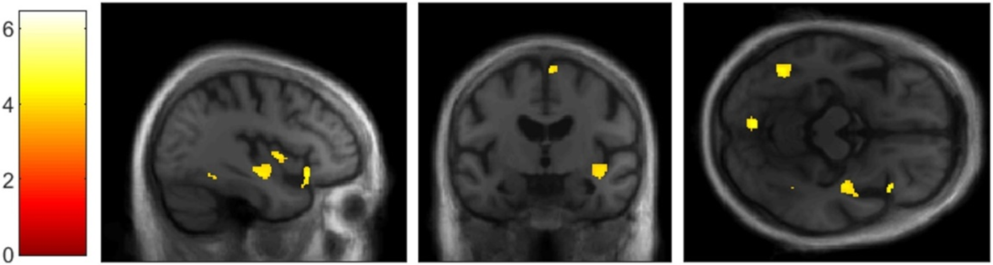
The primary analysis involved the models described above. A sensitivity analysis was also performed looking at the effect of including the MRI image only, the JD image only, or both in the DL model. Due to the training of each DL model taking several days, only one test fold was used in the sensitivity analysis. To improve model interpretability, canonical patterns of brain atrophy for the DL model were identified. Brain atrophy patterns are individualized in nature, so the block occlusion method was followed whereby parts of the image were systematically set to 0 and model performance was evaluated with these images and compared to images without any occlusion. Performing this procedure by systematically blacking out all parts of the image at different trials results in a whole brain atrophy pattern where it is assumed that regions whose blacking out results in a large decrease in model performance must be important to the DL model [38, 39]. This was done for five non-AD and five early AD individuals. The average of the results from the ten folds and ten individuals were used for the final illustrations.

The performance metric of interest for the binary outcome of four-year progression to AD dementia was area under the receiver operating characteristics curve (AUC) and Matthews correlation coefficient (MCC). For the continuous outcome of four-year cognitive decline, the performance metric of interest was R2.

The model fitting procedure involved first performing 10-fold cross validation on the development set, where the training set was the part of the data used to determine model parameters and the validation set was the part of the development set which was held out during cross validation to evaluate model parameters without looking at the test set. Once model parameters were determined from this internal cross validation procedure, performance was finally evaluated on the previously unseen test set and reported as the mean for the ten folds. Five different BioFINDER test sets were used, using a double cross-validation scheme. External evaluation on ADNI data was performed after all models had been finalized.

Statistically significant differences in demographics were determined using p-values from Fisher’s exact test (sex) or t-test for independent samples (remaining variables). To determine statistically significant differences in performance on the test sets for the different models, the results from the 10 folds were used in a Mann-Whitney U-test using the Scipy library (v. 1.4.1) in Python (v. 3.5). All p-values less than 0.05 were considered significant. Bootstrapping on the test sets was used to estimate 95% confidence intervals (CI).