1 Introduction

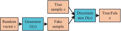
The automobile industry has increasingly prioritized autonomous (González et al., 2015) driving technology due to the ongoing advancements in science and technology. The implementation of driverless vehicles heavily relies on integrating an autonomous driving navigation system, a fundamental component. Analyzing environmental data enables autonomous driving navigation using numerous sensors and algorithms. The utilization of machine learning enables the application of learning-based techniques in making autonomous driving decisions. Imitation learning is often regarded as the prevailing approach when driving regulations are acquired automatically through the analysis of expert driving data. Nevertheless, imitation learning is not without its limitations. Firstly, acquiring substantial quantities of authentic, contemporaneous driving data from proficient experts is a prerequisite, a process that might incur significant costs and consume considerable time. Furthermore, the limited learning capacity of the system restricts its ability to acquire driving skills beyond those displayed in the dataset. Consequently, this limitation may give rise to safety concerns as the system may not possess the necessary knowledge to handle hazardous scenarios not encompassed within the dataset. Thirdly, it is improbable that the imitation learning strategy may surpass human performance, given that the human driving expert assumes the role of a learning supervisor. Given these constraints, it is imperative to investigate alternative methodologies for decision-making in autonomous driving. One such method is reinforcement learning, which automatically enhances and discovers new policies without manual design.

In autonomous driving navigation, reinforcement learning (Kiran et al., 2021; Ye et al., 2021) can help vehicles learn optimal navigation policies by interacting with the road environment. Through continuous trial and error and reward mechanisms, reinforcement learning algorithms can enable vehicles to gradually learn to deal with various complex traffic situations and road conditions. Establishing a suitable reward system is of utmost importance in the context of reinforcement learning for self-driving navigation (Morales et al., 2021). Reinforcement learning algorithms can effectively guide the vehicle to acquire appropriate behavior by employing positive rewards, such as completing the navigation job, or negative rewards, such as contravening traffic regulations. The field of autonomous driving is advancing quickly, with reinforcement learning showing promise in enabling agents to learn how to drive without relying on expert data or manual design. This method entails the agent learning to make decisions in various scenarios, including hazardous ones, potentially surpassing the skills of even the most experienced human drivers. By harnessing the power of reinforcement learning, autonomous driving systems can become more sophisticated and better equipped to handle the intricacies of real-world driving situations.

Nevertheless, implementing reinforcement learning in autonomous driving navigation has certain hurdles. Training (Kaelbling et al., 1998) effective policies is a formidable task primarily because of the intricacies associated with the infinite-dimensional space. Furthermore, complicated and uncertain road environments further compound the challenges in making navigation decisions. The substantial quantity of necessary exploration impedes the practical implementation of large action spaces. This circumstance will result in unsatisfactory outcomes of reinforcement learning-driven policy learning for complex real-world tasks. The occlusion and noise experienced by the sensors hinder the Agent's capacity to perceive the actual status of the surroundings accurately. The Agent cannot reach an optimal conclusion given the existing situation, which is untrue. Most current methodologies employ front-view images as input for end-to-end learning policies. This methodology results in highly complex and dimensional visual characteristics. Another study area that deserves attention is the application of deep reinforcement learning in autonomous Driving. Using elementary deep reinforcement learning methods, such as DQN (Mnih et al., 2013, 2015), may provide limitations in addressing intricate navigation challenges. In recent times, there has been notable progress in developing deep reinforcement learning algorithms with increased efficacy. Autonomous driving technology has limitations that restrict its use to only a few tasks.

This study introduces a novel technique called deep reinforcement learning navigation via decision transformer (DRLNDT). The Transformer model uses the Soft Actor-Critic approach to gain accurate information about the present state by considering the past trajectory state. This method helps the Agent avoid misinterpretations or incorrect judgments regarding the surroundings, possibly due to sensor occlusion or noise. The conventional reinforcement learning model is constructed within the Markov Decision Process (MDP) framework. Our methodological approach is based on the Partially Observable Markov Decision Process (POMDP). The data collected (Ghosh et al., 2021) by the Agent's sensor may need to be more accurate as it depends on a hidden variable that existed in the past state of the sensor and may not accurately represent the current environmental conditions. High-quality images are crucial for capturing a complete and accurate representation of reality and extracting valuable information. Because images of high-quality and larger dimensions can more precisely depict the real world, providing a more comprehensive range of valuable data. Nevertheless, utilizing high-resolution images (Nair et al., 2015; Andrychowicz et al., 2020; Janner et al., 2021) containing intricate visual features results in the intricacy of sample learning and the occupation of substantial memory space, resulting in ineffective learning and inadequate algorithm training. This study uses a variational autoencoder (VAE) to extract latent vectors from high-resolution photos. These latent vectors are then substituted for the original high-resolution images, reducing dimensionality while preserving the salient features of the samples to the greatest extent possible. In addition, we utilize tricks of the Soft Actor-Critic (SAC) policy, including changing temperature and variable learning rate, among others, to enhance the algorithm's efficacy. The conclusive experimental findings demonstrate that our method outperforms the baseline algorithm.

In this paper, we provide the following contributions:

1. In this study, we provide a novel algorithm named deep reinforcement learning navigation via decision transformer (DRLNDT), which leverages a transformer model to acquire knowledge of the current state based on past states. The primary objective of this approach is to mitigate judgment errors that arise due to sensor noise or occlusion in a singular state.

2. The variational autoencoder (VAE) extracts latent vectors from high-quality images, reducing the dimensionality of the state space while preserving essential image properties. In conclusion, optimizing image memory allocation has improved training efficiency and outcomes.

3. The method enables an autonomous vehicle to navigate visually from its starting point to its destination without relying on route direction or high-precision maps, utilizing only high-quality monocular raw photos and producing successful outcomes.

4. Our study incorporates vector states such as velocity and position, which can be effortlessly obtained from the vehicle's intrinsic sensors. Furthermore, we introduce latent vectors from high-quality images to construct a multimodal state space. This method enables the agents to evaluate the current trajectory based on the states, leading to improved overall performance outcomes.

This paper is organized into several sections, each with a specific focus. Section 2 of this paper focuses on the elucidation and explication of pertinent research in the field of autonomous driving. The text emphasizes reinforcement learning techniques used in autonomous driving and the approaches to address POMDPs through reinforcement learning algorithms. Section 3 of this paper introduces various forms and definitions intended to facilitate the comprehension and contextualization of the content. This particular section holds significant importance as it establishes the fundamental basis for the methodology put forth in Section 4. Section 4 of this paper introduces the DRLNDT algorithm, which serves as the central focus of the study and encompasses the most intricate technical aspects. Section 5 depicts the experimental outcomes obtained by implementing our algorithm on the CARLA platform. The results substantiate the superiority of our approach over the baseline approach. The available evidence adequately supports the efficacy of our approach. In conclusion, Section 6 summarizes the essential findings and offers suggestions for future research directions.

2 Related works

We reviewed recent literature on “Reinforcement learning-based autonomous driving” and “Deep reinforcement learning for POMDPs,” summarizing their research.

2.1 Reinforcement learning-based autonomous driving

Kendall et al. (2019) demonstrated the application of deep reinforcement learning to autonomous driving, where a model uses a single monocular image as input to learn a lane following policy. The model is trained through several rounds with randomly initialized parameters. The reward is the distance the vehicle travels without the driver's intervention. The approach relies on continuous, model-free deep reinforcement learning, with all exploration and optimization taking place in the vehicle.

Chen et al. (2019) and his team have developed a framework for deep reinforcement learning in urban autonomous driving scenarios. The framework uses a bird's-eye view and visual coding to capture low-dimensional latent states. The team implemented several state-of-the-art model-free deep RL algorithms in the framework and improved their performance. They tested the performance of the framework in the challenging task of navigating a circular intersection with dense surrounding vehicles and found that it performed excellently compared to the baseline. Additionally, the team introduced and tested three model-free deep RL algorithms to evaluate their success rate in the roundabout intersection task. The results demonstrate the effectiveness of the proposed framework and algorithms in solving complex urban driving tasks.

Liang et al. (2018) present a new Controllable Imitation Reinforcement Learning (CIRL) model for DRL-based autonomous vehicle driving in a high-fidelity vehicle fidelity simulator. CIRL combines Controllable Imitation Learning with DDPG policy learning to address sample inefficiency in reinforcement learning. It outperforms previous approaches, achieving state-of-the-art driving performance on the CARLA benchmark. The CIRL model optimizes the policy network with specialized steering angle rewards for targeting different driving scenarios. It has excellent generalization capabilities across various environments and conditions.

Anzalone et al. (2022) propose a reinforcement curriculum learning method for training agents in a driving simulation environment. The Agent has two phases of training. In the first phase, it starts from a fixed location and drives according to the speed limit without any traffic. In the second phase, the Agent encounters diverse starting locations and randomly generated pedestrians. The driving policy is evaluated quantitatively and qualitatively.

Ozturk et al. (2021) propose the use of curriculum reinforcement learning for autonomous driving in different road and weather conditions. This study tackled the challenge of tuning Agents for optimal performance and generalization in various driving scenarios by using curriculum reinforcement learning. Results showed significant improvement in performance and a reduction in sample complexity. Different courses provided different benefits, indicating potential for future research in automated curriculum training.

Yeom (2022) propose a deep reinforcement learning (DRL) based collision-free path planning architecture for mobile robots, which can navigate unknown environments without supervision. The architecture uses DRL to figure out the unknown environment and predicts control parameters for the mobile robots in the next time step. Experimental results show that the proposed architecture can successfully solve complex navigation problems in dynamic environments.

We found that although all of these studies had some achievements, they did not achieve the task of navigating from the initial position to the termination position. Forward-looking images were used in some methods, but most were low-resolution for algorithm convenience. High-quality images are necessary for more features and real-world applications. Most navigation agents use routing, which the original project did not intend. Routing guides the optimal policy but is not always optimal. Computation needs a high-precision map, which increases costs. It goes against the original project's idea of minimizing the need for high-precision maps.

2.2 Deep reinforcement learning for POMDPs

Heess et al. (2015) used neural networks to solve continuous control problems, and the method was successful in fully observed states. Control problems in real-world scenarios are often only partially observed due to various factors, such as sensor limitations, changes in the controlled object that go unnoticed, or state aliasing caused by function approximation. This article proposes the use of recurrent neural networks trained with temporal backpropagation in model-free continuous control algorithms to tackle partially observed domains.

Igl et al. (2018) proposed a method called Deep Variational Reinforcement Learning (DVRL) to address the challenges of partially observable sequential decision problems. This method helps the agent learn a generative model of the environment and efficiently aggregate information. Researchers developed an n-step approximation of ELBO and a policy for the control task. DVRL outperforms previous approaches and accurately approximates the confidence distribution on latent states. Additionally, a second RNN summarizes the set of particles, accounting for the uncertainty of the latent state after the following action.

Zhu et al. (2017) proposed a new method called Action Specific Deep Recurrent Q Network (ADRQN) to improve the learning performance in partially observable domains. This proposed method encodes actions with a multilayer perceptron (MLP) and combines them with observation features from a convolutional neural network (CNN) to create action-observation pairs. These pairs generate a time series integrated by a Long Short-Term Memory (LSTM) layer to infer latent states. A fully connected layer computes the Q-value, predicting expected rewards for actions in a given state. Tested in partially observable domains, including Atari, this method outperformed state-of-the-art methods.

Hausknecht and Stone (2015) replaced the first fully connected layer of a Deep Q Network (DQN) with an LSTM to add loops and investigated its effect. DRQN, a Deep Recurrent Q Network, integrates temporal information and performs as well as DQN on a standard and partially observed Atari game. Its performance varies with observability and degrades less than DQN when evaluated with partial observations. Looping is a viable alternative to stacking frame histories in the DQN input layer and adapts better to changes in observation quality when evaluated. However, looping does not provide any systematic benefits over stacking observations in the input layer of a convolutional network for non-flickering games.

Chen et al. (2021) use transformer to model high-dimensional distributions of semantic concepts and their latent application to sequential decision problems formalized as reinforcement learning (RL). A new approach for Reinforcement Learning (RL) policy training has been proposed, which uses sequential modeling objectives to train Transformer models with experience data. The architecture, called Decision Transformer, can transform RL problems into conditional sequence modeling. It has been shown to perform well on Atari, OpenAI Gym, and Key-to-Door tasks.

These methods are very inspiring, and we have proposed the DRLNDT method to enable autonomous driving navigation. The transformer model is utilized to learn the actual state from the historical data, thus reducing decision errors caused by object occlusion or sensor noise. The results of our method are better than those of the Baseline method in CARLA.

3 Backgrounds

The Partially Observable Markov Decision Process (POMDP) is a type of sequential decision-making problem that involves modeling the environment based on its location while also considering incomplete and noisy observations. This paper presents a novel approach known as deep reinforcement learning navigation via decision transformer (DRLNDT). The proposed method incorporates a Decision Transformer, which learns the state based on past observations. It then utilizes this learned information to guide the Agent in navigating the task, following a reward learning scheme, from the initial to the termination position. Variable Autoencoder (VAE) (Loaiza-Ganem and Cunningham, 2019; Wei et al., 2020) is a neural network type that can learn a compressed representation of input data by encoding it into the status space and decoding it back into the original space. This paper employs the variational autoencoder (VAE) to enhance the algorithm's performance. DRLNDT utilizes a Transformer neural network architecture to capture temporal dependencies within observations and actions effectively. This capability enhances self-driving vehicles' decision-making process in partially observable urban environments. The paper introduces the Transformer algorithm, integrated with a reinforcement learning algorithm. The reinforcement learning algorithm employs a variational autoencoder (VAE) for compressive characterization of the image data. Next, integrating multimodal observations' time series is performed using the Transformer model. The latent state is acquired by the layer, which subsequently employs the fully connected layer to estimate the value and policy functions, similar to standard reinforcement learning algorithms.

3.1 Markov decision processes

A sequential decision (Arulkumaran et al., 2017) problem refers to a scenario in which an agent is tasked with making a sequence of decisions over time, where each decision's outcome impacts the subsequent decisions. In these types of problems, it is common for the Agent to possess knowledge of the dynamic model of the environment, which implies that the Agent has access to information regarding how the environment will change in response to its actions. In order to establish a formal framework for addressing these issues, researchers employ a mathematical construct known as a Markov Decision Process (MDP) (Puterman, 2014), defined by a 4-tuple denoted as < S, A, P, R >. Here. S represents the set of all possible states in the environment, A represents the set of possible actions the Agent can take, P represents the probability distribution of the next state given the current state and action, and R represents the mapped reward function where each state-action pair is rewarded with a scalar value. During each iteration, the Agent makes a decision by selecting an action at from a set of possible actions A, based on the current state st from a set of possible states S, and its policy π which maps states to actions. As a consequence of this action, the Agent receives an immediate reward rt that is drawn from a distribution R(st, at). Additionally, the Agent transitions to a new state st+1, which is sampled from the probability distribution P(st+1|st, at). The policy π(at|st) is utilized to calculate the state and state-action marginals, which are represented as ρπ(st) and ρπ(st, at), respectively. The margins in question denote the likelihood of being in a specific state or state-action pair under the policy denoted as π. The objective of reinforcement learning is to identify the optimal policy that maximizes the expected discounted reward Rt. The discount factor γ, which falls within the range of [0, 1], determines the relative significance of immediate rewards compared to future rewards.

Rt=rt+γrt+1+γ2rt+2+…    (1)

The discount rewards are computed using Equation (1), which provides a concise representation of the rewards acquired at each time, considering the discount factor associated with each timestep. In the context of Markov Decision Processes (MDPs), the determination of the optimal policy can be achieved through the process of value iteration. This iterative procedure entails the updating of the value function, which serves as a representation of the expected discounted reward for each state given a specific policy.

3.2 Soft Actor Critic

The Q-learning (Watkins and Dayan, 1992) technique was introduced by Watkins and Dayan in 1992 as a solution to reinforcement learning problems characterized by unknown environmental dynamics. The technique is considered model-free as it does not necessitate prior knowledge of the environment or its dynamics. Q-learning aims to estimate the value associated with executing an action and adhering to an optimal policy π within a specific state. The quantity above is commonly referred to as the state-action value or, more succinctly, the Q-value. The Q-value measures the anticipated total reward achieved by selecting a specific action in a given state and adhering to the optimal policy. The Q-value is defined recursively as the summation of the immediate reward acquired from the action and the discounted value of the subsequent state-action pair. The utilization of a discount factor γ, which falls within the range of [0, 1], serves the purpose of discounting future rewards and facilitating the convergence of Q values. The optimal policy π* can be derived by selecting the action with the maximum Q-value in every state. Q-learning is an algorithm that operates off-policy, meaning it learns the Q-value of a target policy while adhering to various behavioral policies.

The function Qπ(s, a) is a formal mathematical representation denoting the expected collect reward that an Agent obtains when it selects action a within state s and adheres to policy π. The Q-value is acquired through an iterative process, wherein the Agent continually updates its estimate of the Q-value by considering the rewards it obtains during its interactions with the environment.

Qπ(s,a)=Eπ(Rt|st=s,at=a)    (2)

The Equation (2) represents the anticipated reward that the Agent is expected to obtain at a given time t, under the condition that the Agent is in a specific state denoted as s and selects a particular action denoted as a, by the policy denoted as π. Q-values play a crucial role in reinforcement learning, enabling the Agent to make optimal action selections within a specific state. The Agent selects the action with the highest Q value within the given state. The process of updating Q-values can be accomplished through the utilization of a method known as Q learning. This technique entails the modification of the Q-value associated with the present state-action pair by considering the highest Q-value among the subsequent state-action pairs. The Q-learning algorithm is classified as an off-policy method, which implies that the Agent can learn the optimal Q-value even when it adheres to a policy that differs from the one being evaluated. The Q-value is employed for approximating the value of the policy, specifically the anticipated cumulative reward that the Agent will obtain by adhering to the policy. The maximization of the value function determines the optimal policy.

The Q function is a mathematical function that provides an estimation of the expected future reward when a specific action is taken within a specific state in Equation (3).

Q(s,a)=Q(s,a)+β(r+γmaxa′Q(s′,a′)-Q(s,a))    (3)

The equation presented herein represents the Q-learning update rule, which is a fundamental element of numerous reinforcement learning algorithms. The equation incorporates various components, namely the current state (s), the action taken (a), the reward received (r), the subsequent state (s′), and a discount factor (γ). This equation updates the Q value of the current state-action pair by adding the scaling difference between the estimated Q value of the following state-action pair and the Q value of the current state-action pair. The scaling factor β is the learning rate, which determines how much new information is incorporated into existing estimates. In instances with many states where it is impossible to save Q values for all state-action combinations, the equation above is used. In contrast, a function approximator, such as a neural network, estimates the Q values for previously unobserved state-action combinations. The DQN method illustrates a reinforcement learning methodology that utilizes a neural network to estimate Q values. Using the current state and action as input variables, the neural network, identified by the parameter θ, generates an estimated value Q for a specific state-activity combination.

In contrast to the DQN algorithm, Soft Actor-Critic (SAC) (Haarnoja et al., 2018) is an off-policy Actor-Critic algorithm that operates within a maximum entropy reinforcement learning framework. The primary objective of SAC is to optimize both the expected return and entropy. SAC contains several modifications to accelerate training and enhance the stability of hyperparameters, such as automatic tuning of the constraint formulas for the temperature hyperparameter. The maximum entropy objective extends the conventional aim employed in conventional reinforcement learning methods. Adding an entropy element to the objective signifies that the optimal policy seeks to maximize its entropy at each accessed state.

π*=argmaxπ ∑tE(st,at)~ρπ[r(st,at)+αH(π(·|st))]    (4)

Maximizing the expected reward and entropy of each state determines the optimal policy. The parameter α in the Equation (4) governs the relative significance of the entropy term concerning the reward, influencing the optimal policy's probabilistic characteristics. The maximum entropy aim applies when the best policy necessitates randomization or stochasticity, such as in exploration tasks or when confronted with unpredictable settings. The discount factor, denoted as γ, is a scalar within the range of 0 to 1, which plays a crucial role in determining the relative significance of future rewards within the context of decision-making. A discount factor of zero implies that only incentives in the present period are considered. In contrast, a discount factor of one indicates that rewards in the future are given equal importance to immediate rewards. The discount factor is crucial in infinite horizon problems since it guarantees the convergence of the expected reward and entropy to a limited value. With the discount factor, the cumulative value of predicted rewards and entropy may remain the same toward infinity, making the objective function's optimization attainable. Incorporating the discount factor enables the algorithm to effectively weigh the significance of immediate benefits against those obtained in the future, facilitating more optimal decision-making over extended time horizons.

Determine the solution for the optimal Q-function, which establishes a correspondence between a state-action pair and a value that denotes the anticipated long-term benefit associated with executing that action in that state and afterward adhering to the optimal policy. From the ideal Q-function, one can deduce the best policy. The suggested algorithm is a Soft Actor-Critic (SAC) approach that is formulated using the policy iteration framework. The Q-function associated with the present policy is assessed, and the policy is then modified through the utilization of off-policy gradient updating. Off-policy suggests a difference between the policy being updated and the policy that produced the data for modification. The Maximum Entropy Reinforcement Learning framework serves as the foundation for the Soft Actor-Critic algorithm, where the Actor's objective is to maximize predicted reward and entropy.

Soft policy iteration is a generalized algorithm for learning optimal maximum entropy policies. The algorithm alternates between policy evaluation and policy improvement in a maximum entropy framework. The derivation of the algorithm is based on a tabular setup that allows for theoretical analysis and convergence guarantees. The algorithm aims to converge to the optimal policy among a set of strategies, which may correspond to a set of parameterized densities. The set of strategies to which the algorithm converges is not fixed and can vary depending on the specific problem to be solved. The algorithm aims to maximize the expected return while maximizing the entropy of the strategies. The entropy of a policy is a measure of the stochasticity of the policy, and maximizing it encourages exploration and prevents the policy from falling into a local optimum. The algorithm is called “Soft” because it uses a Soft-valued function instead of a hard-valued function. Soft-valued functions are smoothed versions of hard-valued functions, which are easier to optimize and prevent overfitting.

Soft policy iteration is a technique employed in the field of reinforcement learning to assess the efficacy of a policy and determine its worth by optimizing the maximum entropy target. During the policy evaluation phase of Soft policy iteration, it is possible to calculate Soft Q values for fixed policy iterations. The computation of the Soft Q value involves the iterative use of the modified Bellman backup operator, denoted as Tπ in Equation (5).

TπQ(st,at)≜r(st,at)+γEst+1~p[V(st+1)]    (5)

where r(st, at) represents the reward obtained for taking an action at in state st, γ represents the discount factor, and p represents the transfer probability distribution. The Soft Q-value is calculated using the Soft state value function V(st) in Equation (6).

V(st)=Eat~π[Q(st,at)-αlogπ(at|st)]    (6)

The value of Q for taking an action at in state st is denoted as Q(st, at). The probability of taking an action in state st according to the policy π is represented as π(at|st). The temperature parameter α regulates the balance between maximizing the expected payoff of the policy and maximizing the entropy. By repeatedly applying the Bellman backup operator T to any initial Q function Q : S × A → R, one can obtain the Soft Q function for any policy π. The Soft Q function is an advantageous instrument for assessing policies in the context of reinforcement learning due to its consideration of policy uncertainty and promotion of exploration.

To create a feasible approximation of the Soft policy iteration, a function approximator can be utilized for the Soft Q function and policy. Instead of assessing and enhancing the convergence aspect, it is suggested to employ stochastic gradient descent as an alternative approach to optimize both networks simultaneously. The Soft Q function and policy are parameterized by a neural network with θ and phi parameters. The Soft Q function can be modeled as an expressive neural network. In contrast, the policy can be modeled as a Gaussian function, with the neural network providing the mean and covariance. The rules for updating these parameter vectors are subsequently derived and employed to optimize the network during the training process. The objective is to tackle the issues of significant sample complexity and vulnerability to hyperparameters commonly observed in model-free deep reinforcement learning methods through the utilization of function approximators and stochastic gradient descent. The suggested methodology is grounded in the framework of maximum entropy reinforcement learning. This paradigm seeks to optimize both the expected return and entropy, enabling the Agent to accomplish the goal while exhibiting a high degree of randomness in its actions.

The Soft Q function is a modified version of the Q function employed in the field of reinforcement learning, which integrates a component of entropy to promote exploration. The parameters of the Soft Q function are optimized through training in order to minimize the Soft Bellman residual, which serves as a metric for quantifying the discrepancy between the anticipated Q value and the real Q value.

JQ(θ)=E(st,at)~D[12(Qθ(st,at)−(r(st,at)                   +γEst+1~p[Vθ¯(st+1)]))2]    (7)

The Soft Bellman residual is formally defined in Equation (7), whereby it encompasses the calculation of the expected value of the squared discrepancy between the predicted Q-value and the summation of the reward and subsequent state discount values. The utilization of the Soft Q function argument serves as an implicit parameterization of the value function, as specified in Equation (6). A crucial component of the SAC algorithm, the value function estimates the expected reward for a given state. The parameters of the Soft Q function are optimized by the utilization of stochastic gradient descent, a widely employed optimization method within the field of deep learning. The optimization of the Soft Q function parameters is a crucial component of the SAC method as it enables the Agent to acquire a precise estimation of the anticipated reward associated with a specific state-action combination. By reducing the residuals of the Bellman Soft equation, the Agent can acquire improved decision-making abilities and attain enhanced performance across a range of reinforcement learning challenges.

∇^θJQ(θ)=∇θQθ(at,st)(Qθ(st,at)−(r(st,at)+γ(Qθ¯(st+1,at+1)                       −αlog(πϕ(at+1|st+1))))    (8)

The Soft Q function arguments, which are obtained from Equation (6), implicitly parameterize the value function. The objective is optimized using stochastic gradient descent, where the stochastic gradient is computed using the gradient of the Q function with respect to its parameters in Equation (8). The Q function is a mathematical function that accepts the current state (st) and action (at) as its input and produces the anticipated reward for that specific state-activity combination. The expected reward is equal to the sum of the instantaneous reward (r(st, at)) and the discounted expected reward (Qθ(st+1, at+1)) for the next state-action pair. The Soft Q function is modified by the addition of a term that promotes exploration, which is determined by the temperature parameter α and the policy function πϕ(at + 1|st + 1). The update also employs a target Soft Q function with parameter θ̄, which is derived as an exponentially shifted mean of the Soft Q function weights. The utilization of this target Q function serves the purpose of stabilizing the training process and mitigating the occurrence of overfitting.

Jπ(ϕ)=Est~D[Eat~πϕ[αlog(πϕ(at|st))-Qθ(st,st)]]    (9)

Equation (9) denotes the goal function Jπ(ϕ) employed for the purpose of acquiring the policy parameters in the Soft Actor-Critic (SAC) algorithm. The objective function Jπ(ϕ) entails the maximization of the ex